
Chapter4 - Induction, Recursion, and Reduction - Part1
Book - Python Algorithms by Magnus Lie Hetland
Chapter 4 - Induction and Recursion … and Reduction
Reduction: A reduction is any algorithm that converts a large data set into a smaller data set using an operator on each element. A simple reduction example is to compute the sum of the elements in an array.
Induction and recursion are, in a sense, mirror images of one another, and both can be seen as examples of reduction. Here’s a quick overview of what these terms actually mean:
- Reduction: means transforming one problem to another. We normally reduce an unknown problem to one we know how to solve. The reduction may involve transforming both the input (so it works with the new problem) and the output (so it’s valid for the original problem).
- Induction, or mathematical induction: is used to show that a statement is true for a large class of objects (often the natural numbers). We do this by first showing it to be true for a base case (such as the number 1) and then showing that it “carries over” from one object to the next; for example, if it’s true for n–1, then it’s true for n.
- Recursion: is what happens when a function calls itself. Here we need to make sure the function works correctly for a (nonrecursive) base case and that it combines results from the recursive calls into a valid solution.
Both induction and recursion involve reducing (or decomposing) a problem to smaller subproblems and then taking one step beyond these, solving the full problem.
In short, start to solve a smaller problem then expand it incremently to the large value.
Let’s take an example.
You have a list of numbers, and you want to find the two (nonidentical) numbers that are closest to each other (that is, the two with the smallest absolute difference):
from random import randrange
import time
start = time.time()
seq = [randrange(10**10) for i in range(100)]
dd = float("inf")
for x in seq:
    for y in seq:
        if x == y: continue
        d = abs(x-y)
        if d < dd:
            xx, yy, dd = x, y, d
dd = float("inf")
for i in range(len(seq)-1):
    x, y = seq[i], seq[i+1]
    if x == y: continue
    d = abs(x-y)
    if d < dd:
        xx, yy, dd = x, y, d
result:
Quadratic : 0.01048
Loglinear : 0.00035
Our original problem was “Find the two closest numbers in a sequence,” and we reduced it to “Find the two closest numbers in a sorted sequence,” by sorting seq. In this case, our reduction (the sorting) won’t affect which answers we get. In general, we may need to transform the answer so it fits the original problem.
For example, let’s say we’re investigating the sum of the first n odd numbers; \(P(n)\) could then be the following statement:
\[ 1+3+5+\cdot\cdot\cdot+(2n-3)+(2n-1) = n^{2}\]
We’re assuming the following \(P(n-1)\):
\[ 1+3+5+\cdot\cdot\cdot+(2n-3) = (n-1)^{2}\]
We can deduce \(P(n)\):
\(\begin{align}
1+3+5+\cdot\cdot\cdot+(2n-3)+(2n-1) & = (n-1)^{2} + (2n-1) \\
& = (n^{2}-2n+1) + (2n-1) \\
& = n^{2} \\
\end{align}\)
And there you go. The inductive step is established, and we now know that the formula holds for all natural numbers n.
Check Board
Now, consider the following classic puzzle. How do you cover a checkerboard that has one corner square missing, using L-shaped tiles, as illustrated in Figure 4-2? Is it even possible? Where would you start? You could try a brute-force solution, just starting with the first piece, placing it in every possible position (and with every possible orientation), and, for each of those, trying every possibility for the second, and so forth. That wouldn’t exactly be efficient. How can we reduce the problem? Where’s the reduction?
[Figure 4-2]
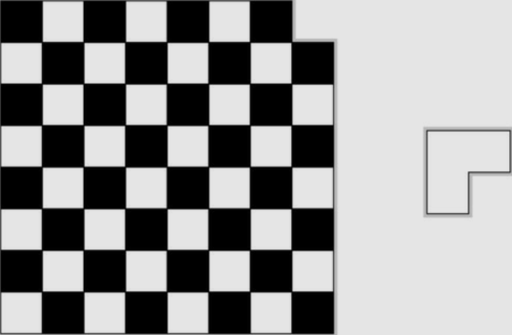
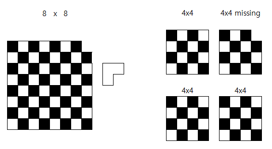
The question is how we can carve up the board into smaller ones of the same shape. It’s quadratic, so a natural starting point might be to split it into four smaller squares. The only thing standing between us and a complete solution at that point is that only one of the four board parts has the same shape as the original, with the missing corner. The other three are complete (quarter-size) checkerboards. That’s easily remedied, however. Just place a single tile so that it covers one corner from each of these three subboards, and, as if by magic, we now have four subproblems, each equivalent to (but smaller than) the full problem!
To clarify the induction here, let’s say you don’t actually place the tile quite yet. You just note which three corners to leave open. By the inductive hypothesis, you can cover the three subboards (with the base case being four-square boards), and once you’ve finished, there will be three squares left to cover, in an L-shape. The inductive step is then to place this piece, implicitly combining the four subsolutions. Now, because of induction, we haven’t only solved the problem for the eight-by-eight case; the solution holds for any board of this kind, as long as its sides are (equal) powers of two.
In induction, we (conceptually) start with a base case and show how the inductive step can take us further, up to the full problem size, n. Recursion usually seems more like breaking things down. You start with a full problem, of size n. You delegate the subproblem of size n–1 to a recursive call, wait for the result, and extend the subsolution you get to a full solution. In a way, induction shows us why recursion works, and recursion gives us an easy way of (directly) implementing our inductive ideas.
IMPLEMENTING THE CHECKERBOARD COVERING
def cover(board, lab=1, top=0, left=0, side=None):
    if side is None:
        side = len(board) # Side length of subboard:
    s = side // 2 # Offsets for outer/inner squares of subboards:
    offsets = (0, -1), (side-1, 0)
    for dy_outer, dy_inner in offsets:
        for dx_outer, dx_inner in offsets:
            # If the outer corner is not set...
            if not board[top+dy_outer][left+dx_outer]:
                # ... label the inner corner:
                board[top+s+dy_inner][left+s+dx_inner] = lab
    # Next label:
    lab += 1
    if s > 1:
        for dy in [0, s]:
            for dx in [0, s]:
                # Recursive calls, if s is at least 2:
                lab = cover(board, lab, top+dy, left+dx, s)
    # Return the next available label:
    return lab
The main work in the function is checking which of the four center squares to cover with the L-tile. We cover only the three that don’t correspond to a missing (outer) corner. Finally, there are four recursive calls, one for each of the four subproblems. (The next available label is returned, so it can be used in the next recursive call.) Here’s an example of how you might run the code:
>>> board = [[0]*8 for i in range(8)] # Eight by eight checkerboard
>>> board[7][7] = -1 # Missing corner
>>> cover(board)
22
>>> for row in board:
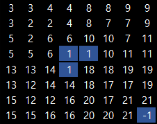
... print((" %2i"*8) % tuple(row))
3 3 4 4 8 8 9 9
3 2 2 4 8 7 7 9
5 2 6 6 10 10 7 11
5 5 6 1 1 10 11 11
13 13 14 1 18 18 19 19
13 12 14 14 18 17 17 19
15 12 12 16 20 17 21 21
15 15 16 16 20 20 21 -1
You can see -1 and 1’s in the middle of 8x8 checkboard. By putting a L-shape tile in the middle, the splited three 4x4 checkboard are having the same solution as with the first 4x4 checkboard with -1 at the corner.
Solving subproblems of 4 of 4x4 checkboard
Thinking recursively, Implement iteratively
A sorting problem.
Reduction: reduce the problem by one element(n-1).
Either we can assume (inductively) that the first n–1 elements are already sorted and insert element n in the right place, or we can find the largest element, place it at position n, and then sort the remaining elements recursively.
The former gives us insertion sort, while the latter gives selection sort.
Insertion Sort & Selection Sort
To get the sequence sorted up to position \(i\), first sort it recursively up to position \(i–1\) (correct by the induction hypothesis) and then swap element \(seq[i]\) down until it reaches its correct position among the already sorted elements.
The base case is when i = 0; a single element is trivially sorted. If you wanted, you could add a default case, where i is set to len(seq)-1.
Instead of recursing backward, it iterates forward, from the first element. so the behaviors of the two versions are identical.
# Recursive Insersion Sort
def ins_sort_rec(seq, i):
    if i==0: return                             # Base case -- do nothing
    ins_sort_rec(seq, i-1)                      # Sort 0..i-1
    j = i                                       # Start "walking" down
    while j > 0 and seq[j-1] > seq[j]:          # Look for OK spot
        seq[j-1], seq[j] = seq[j], seq[j-1]     # Keep moving seq[j] down
        j -= 1                                  # Decrement j
# Iterative Insertion Sort
def ins_sort(seq):
    for i in range(1,len(seq)):                 # 0..i-1 sorted so far
        j = i                                   # Start "walking" down
        while j > 0 and seq[j-1] > seq[j]:      # Look for OK spot
            seq[j-1], seq[j] = seq[j], seq[j-1] # Keep moving seq[j] down
            j -= 1                              # Decrement j
# Recursive Selection Sort
def sel_sort_rec(seq, i):
    if i==0: return                             # Base case -- do nothing
    max_j = i                                   # Idx. of largest value so far
    for j in range(i):                          # Look for a larger value
        if seq[j] > seq[max_j]: max_j = j       # Found one? Update max_j
    seq[i], seq[max_j] = seq[max_j], seq[i]     # Switch largest into place
    sel_sort_rec(seq, i-1)                      # Sort 0..i-1
# Iterative Selection Sort
def sel_sort(seq):
    for i in range(len(seq)-1,0,-1):            # n..i+1 sorted so far
        max_j = i                               # Idx. of largest value so far
        for j in range(i):                      # Look for a larger value
            if seq[j] > seq[max_j]: max_j = j   # Found one? Update max_j
        seq[i], seq[max_j] = seq[max_j], seq[i] # Switch largest into place
Why iterative implementation is superior to recursive one?
- less overhead with iterative way. (faster)
- recursion has a limit of maximum stack depth in most languages. (Runtime Error)
Tail Recursion Optimization
Every time call recursion, the stack keeps increasing the depth of the stack.
Two options to solve this:
- Use iterative solution
- Use tail recursion elimination or tail recursio optimization that
Tail calls can be implemented without adding a new stack frame to the call stack. Producing such code instead of a standard call sequence is called tail call elimination or tail call optimization. (wikipedia)
Tail call elimination: https://en.wikipedia.org/wiki/Tail_call
Tail recursion: http://philosophical.one/posts/tail-recursion-in-python/
Leave a comment