Chapter4 - Induction, Recursion, and Reduction - Part2

Book - Python Algorithms by Magnus Lie Hetland

Chapter 4 - Induction and Recursion … and Reduction

Designinig with Induction

About three problems:

• Matching problem
• The celebrity problem
• Topological Sort

Matching Problem: Finding a Maximum Permutation

Find a way to let them switch seats to make as many people as possible happy with the result. This is a form of matching problem. We can model the problem (instance) as a graph.

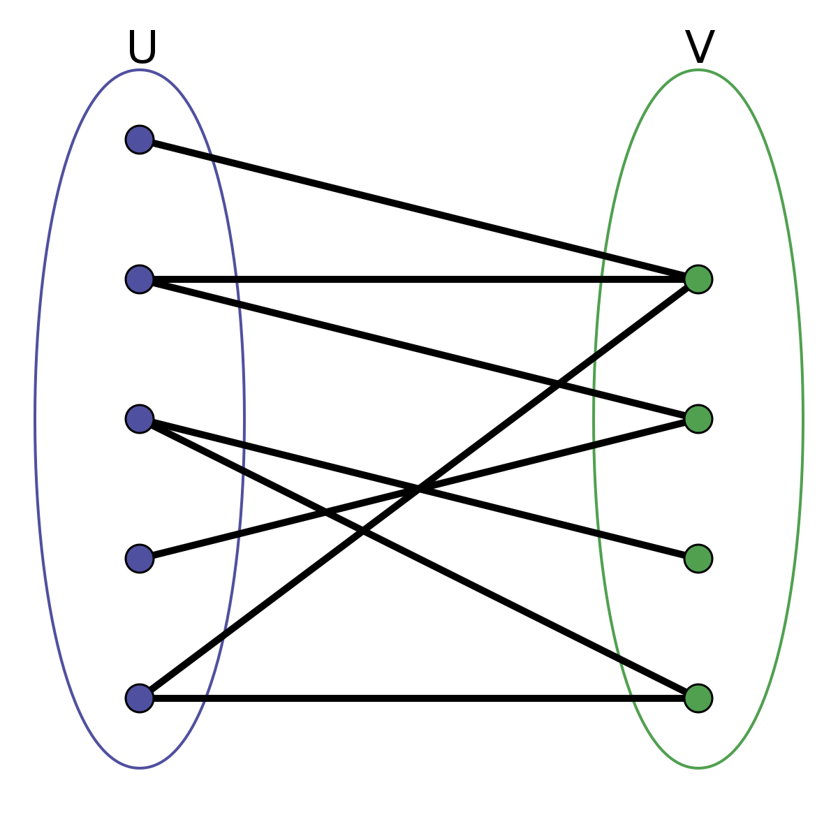
This is an example of what’s called a bipartite graph, which means that the nodes can be partitioned into two sets, where all the edges are between the sets (and none of them inside either). In other words, you could color the nodes using only two colors so that no neighbors had the same color.

Bipartite Graph(이분 그래프): 그래프 이론에서, 이분 그래프란 모든 꼭짓점을 빨강과 파랑으로 색칠하되, 모든 변이 빨강과 파랑 꼭짓점을 포함하도록 색칠할 수 있는 그래프이다. (wikipedia)

Simple-bipartite-graph

Formalize the problem.
In this case, we want to let as many people as possible get the seat they’re “pointing to.” The others will need to remain seated. Another way of viewing this is that we’re looking for a subset of the people (or of the pointing fingers) that forms a one-to-one mapping, or permutation. This means that no one in the set points outside it, and each seat (in the set) is pointed to exactly once. That way, everyone in the permutation is free to permute—or switch seats—according to their wishes. We want to find a permutation that is as large as possible (to reduce the number of people that fall outside it and have their wishes denied).

Our first step to ask:
Where is the reduction?
How can we reduce the problem to a smaller one?
What subproblem can we delegate (or recursively) or assume (inductively) to be solved already?

With induction, see whether we can shrink the problem from \(n\) to \(n-1\). The inductive assumption follows from our general approach. We simply assume that we can solve the problem (that is, find a maximum subset that forms a permutation) for \(n-1\) people. The only thing that requires any creative problem solving is safely removing a single person so that the remaining subproblem is one that we can build on (that is, one that is part of a total solution).

If each person points to a different seat, the entire set forms a permutation, which must certainly be as big as it can be—no need to remove anyone because we’re already done.
The base case is also trivial. For n = 1, there is nowhere to move. So, let’s say that n > 1 and that at least two persons are pointing to the same seat (the only way the permutation can be broken).

Figure 4-4
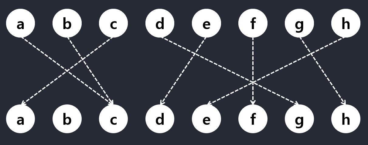Take a and c in Figure 4-4, for example. They’re both pointing to c, and we can safely say that one of them must be eliminated. However, which one we choose is crucial.
Say, for example, we choose to remove a (both the person and the seat). We then notice that c is pointing to a, which means that c must also be eliminated. Finally, b points to c and must be eliminated as well—meaning that we could have simply eliminated b to begin with, keeping a and c (who just want to trade seats with each other).

After removing a, all a, b, and c should be eliminated.

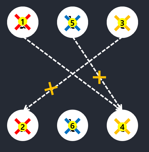
When looking for inductive steps like this, it can often be a good idea to look for something that stands out. What, for example, about a seat that no one wants to sit in (that is, a node in the lower row in Figure 4-4 that has no in-edges)? In a valid solution (a permutation), at most one person (element) can be placed in (mapped to) any given seat (position). That means there’s no room for empty seats, because at least two people will then be trying to sit in the same seat. In other words, it is not only OK to remove an empty seat (and the corresponding person); it’s actually necessary.

Therefore, we can eliminate b, and what remains is a smaller instance (with n = 7) of the same problem , and, by the magic of induction, we’re done!
Or are we? We always need to make certain we’ve covered every eventuality. Can we be sure that there will always be an empty seat to eliminate, if needed? Indeed we can. Without empty seats, the n persons must collectively point to all the n seats, meaning that they all point to different seats, so we already have a permutation.

In short:

• If no empty seats, all members are pointing different seats meaning that we already have a permutation. Done!
• If empty seats, remove an empty seat and the corresponding member

Now, implementing.

>>> M = [2, 2, 0, 5, 3, 5, 7, 4] 
>>> M[2] # c is mapped to a 
0

A Naïve Implementation of the Recursive Algorithm Idea for Finding a Maximum Permutation

def naive_max_perm(M, A=None): 
    if A is None:                               # The elt. set not supplied? 
        A = set(range(len(M)))                  # A = {0, 1, ... , n-1} 
    if len(A) == 1: return A                    # Base case -- single-elt. A 
    B = set(M[i] for i in A)                    # The "pointed to" elements 
    C = A - B                                   # "Not pointed to" elements 
    if C:                                       # Any useless elements? 
        A.remove(C.pop())                       # Remove one of them 
        return naive_max_perm(M, A)             # Solve remaining problem 
    return A                                    # All useful -- return all

The function naive_max_perm receives a set of remaining people (A) and creates a set of seats that are pointed to (B). If it finds an element in A that is not in B (variable C), it removes the element and solves the remaining problem recursively. Let’s use the implementation on our example, M.

>>> naive_max_perm(M) 
{0, 2, 5}

So, a, c, and f can take part in the permutation. The others will have to sit in nonfavorite seats.
The handy set type lets us manipulate sets with ready-made high-level operations, rather than having to implement them ourselves.
There are some problems, though. For one thing, we might want an iterative solution. This is easily remedied—the recursion can quite simply be replaced by a loop (like we did for insertion sort and selection sort). A worse problem, though, is that the algorithm is quadratic!
The most wasteful operation is the repeated creation of the set B. If we could just keep track of which chairs are no longer pointed to, we could eliminate this operation entirely. One way of doing this would be to keep a count for each element. We could decrement the count for chair x when a person pointing to x is eliminated, and if x ever got a count of zero, both person and chair x would be out of the game.

Reference Counting: It’s a basic component in many systems for garbage collection that automatically deallocates objects that no longer useful.

If we needed to make sure the elements were eliminated in the order in which we discover that they’re no longer useful, we would need to use a first-in, first-out queue such as the deque class giving us less overhead.

def max_perm(M): 
    n = len(M)                                  # How many elements? 
    A = set(range(n))                           # A = {0, 1, ... , n-1} 
    count = [0]*n                               # C[i] == 0 for i in A 

    for i in M:                                 # All that are "pointed to" 
        count[i] += 1                           # Increment "point count" 

    Q = [i for i in A if count[i] == 0]         # Useless elements 

    while Q:                                    # While useless elts. left... 
        i = Q.pop()                             # Get one 
        A.remove(i)                             # Remove it 
        j = M[i]                                # Who's it pointing to? 
        count[j] -= 1                           # Not anymore... 

        if count[j] == 0:                       # Is j useless now? 
            Q.append(j)                         # Then deal w/it next 

    return A                                    # Return useful elts.

Counting Sort & Fam

One of the most well-known (and really, really pretty) examples of what counting can do is counting sort. If you can count your elements, you can sort in linear time!

from collections import defaultdict 
def counting_sort(A, key=lambda x: x): 
    B, C = [], defaultdict(list)                # Output and "counts" 
    for x in A: 
        C[key(x)].append(x)                     # "Count" key(x) 
    for k in range(min(C), max(C)+1):           # For every key in the range 
        B.extend(C[k])                          # Add values in sorted order 
    return B

Counting-sort does need more space than an in-place algorithm like Quicksort, for example, so if your data set and value range is large, you might get a slowdown from a lack of memory. This can partly be handled by handling the value range more efficiently. We can do this by sorting numbers on individual digits (or strings on individual characters or bit vectors on fixed-size chunks). If you first sort on the least significant digit, because of stability, sorting on the second least significant digit won’t destroy the internal ordering from the first run. (This is a bit like sorting column by column in a spreadsheet.) This means that for d digits, you can sort n numbers in Θ(dn) time. This algorithm is called radix sort.
Another somewhat similar linear-time sorting algorithm is bucket sort. It assumes that your values are evenly (uniformly) distributed in an interval, for example, real numbers in the interval [0,1), and uses n buckets, or subintervals, that you can put your values into directly. In a way, you’re hashing each value into its proper slot, and the average (expected) size of each bucket is Θ(1). Because the buckets are in order, you can go through them and have your sorting in Θ(n) time, in the average case, for random data.

Radix sort (기수정렬): 기수로는 정수, 낱말, 천공카드 등 다양한 자료를 사용할 수 있으나 크기가 유한하고 사전순으로 정렬할 수 있어야 한다. 버킷 정렬의 일종으로 취급되기도 한다. 기수에 따라 원소를 버킷에 집어 넣기 때문에 비교 연산이 불필요하다. 유효숫자가 두 개 이상인 경우 모든 숫자 요소에 대해 수행될 때까지 각 자릿수에 대해 반복한다. 따라서 전체 시간 복잡도는 \(O(nw)\) (w는 기수의 크기)이 된다. 정수와 같은 자료의 정렬 속도가 매우 빠르다. 하지만, 데이터 전체 크기에 기수 테이블의 크기만한 메모리가 더 필요하다. 기수 정렬은 정렬 방법의 특수성 때문에, 부동소수점 실수처럼 특수한 비교 연산이 필요한 데이터에는 적용할 수 없지만, 사용 가능할 때에는 매우 좋은 알고리즘이다. https://ko.wikipedia.org/wiki/%EA%B8%B0%EC%88%98_%EC%A0%95%EB%A0%AC

Bucket Sort: 배열의 원소를 여러 버킷으로 분산하여 작동하는 정렬 알고리즘이다. 버킷은 빈(bin)이라고도 불리고, 버킷 정렬도 빈 정렬로도 불린다. 각 버킷은 다른 정렬 알고리즘을 사용하거나 버킷 정렬을 반복 적용해 각각 정렬한다. 분포 정렬이고 일반화된 비둘기집 정렬과 같다. 최하위 유효숫자부터 정렬하는 기수 정렬과도 비슷하다. 비교를 이용해 구현할 수도 있어서 비교 정렬 알고리즘으로 보기도 한다. 계산 복잡도는 각 버킷을 정렬하는 데 사용되는 알고리즘, 사용할 버킷 수, 버킷마다 균일한 입력이 들어가는지 여부에 따라 다르다. https://ko.wikipedia.org/wiki/%EB%B2%84%ED%82%B7_%EC%A0%95%EB%A0%AC

Radix Sort:

def countingSort(arr, digit):
    n = len(arr)
  
    # 배열의 크기에 맞는 output 배열을 생성하고 10개의 0을 가진 count란 배열을 생성한다. 
    output = [0] * (n)
    count = [0] * (10)
    
    #digit, 자릿수에 맞는 count에 += 1을 한다. 
    for i in range(0, n):
        index = int(arr[i]/digit) 
        count[ (index)%10 ] += 1
 
    # count 배열을 수정해 digit으로 잡은 포지션을 설정한다.  
    for i in range(1,10):
        count[i] += count[i-1]  
        print(i, count[i])
    # 결과 배열, output을 설정한다. 설정된 count 배열에 맞는 부분에 arr원소를 담는다.   
    i = n - 1
    while i >= 0:
        index = int(arr[i]/digit)
        output[ count[ (index)%10 ] - 1] = arr[i]
        count[ (index)%10 ] -= 1
        i -= 1

    #arr를 결과물에 다시 재할당한다.  
    for i in range(0,len(arr)): 
        arr[i] = output[i]
 
# Method to do Radix Sort
def radixSort(arr):
    # arr 배열중에서 maxValue를 잡아서 어느 digit, 자릿수까지 반복하면 될지를 정한다. 
    maxValue = max(arr)  
    #자릿수마다 countingSorting을 시작한다. 
    digit = 1
    while int(maxValue/digit) > 0: 
        countingSort(arr,digit)
        digit *= 10
 
arr = [ 170, 45, 75, 90, 802, 24, 2, 66]
#arr = [4, 2, 1, 5, 7, 2]
radixSort(arr)
 
for i in range(len(arr)):
    print(arr[i], end=" ")

Bucket Sort:

def bucket_sort(seq):
    # make buckets
    buckets =  [[] for _ in range(len(seq))]
    # assign values
    for value in seq:
        bucket_index = value * len(seq) // (max(seq) + 1)
        buckets[bucket_index].append(value)
    # sort & merge
    sorted_list = []
    for bucket in buckets:
        sorted_list.extend(quick_sort(bucket))
    return sorted_list

def quick_sort(ARRAY):
    ARRAY_LENGTH = len(ARRAY)
    if( ARRAY_LENGTH <= 1):
        return ARRAY
    else:
        PIVOT = ARRAY[0]
        GREATER = [ element for element in ARRAY[1:] if element > PIVOT ]
        LESSER = [ element for element in ARRAY[1:] if element <= PIVOT ]
        return quick_sort(LESSER) + [PIVOT] + quick_sort(GREATER)

The Celebrity Problem

A Naïve Solution to the Celebrity Problem

def naive_celeb(G): 
    n = len(G) 
    for u in range(n):                          # For every candidate... 
        for v in range(n):                      # For everyone else... 
            if u == v: continue                 # Same person? Skip. 
            if G[u][v]: break                   # Candidate knows other 
            if not G[v][u]: break               # Other doesn't know candidate 
        else: 
            return u                            # No breaks? Celebrity! 
    return None                                 # Couldn't find anyone

The idea is as follows: The celebrity knows no one, but everyone knows the celebrity.

The naive_celeb function tackles the problem head on. Go through all the people, checking whether each person is a celebrity. This check goes through all the others, making sure they all know the candidate person and that the candidate person does not know any of them. This version is clearly quadratic, but it’s possible to get the running time down to linear.

The key, as before, lies in finding a reduction—reducing the problem from \(n\) persons to \(n–1\) as cheaply as possible. The naive_celeb implementation does, in fact, reduce the problem step by step. In iteration k of the outer loop, we know that none of \(0...k–1\) can be the celebrity, so we need to solve the problem only for the remainder, which is exactly what the remaining iterations do. This reduction is clearly correct, as is the algorithm. What’s new in this situation is that we have to try to improve the efficiency of the reduction. To get a linear algorithm, we need to perform the reduction in constant time.

To reduce the problem from \(n\) to \(n–1\), we must find a noncelebrity, someone who either knows someone or is unknown by someone else.

And if we check G[u][v] for any nodes u and v, we can eliminate either u or v! If G[u][v] is true, we eliminate u; otherwise, we eliminate v. If we’re guaranteed that there is a celebrity, this is all we need. Otherwise, we can still eliminate all but one candidate, but we need to finish by checking whether they are, in fact, a celebrity, like we did in naive_celeb.

def celeb(G): 
    n = len(G) 
    u, v = 0, 1                                 # The first two 
    for c in range(2,n+1):                      # Others to check 
        if G[u][v]: u = c                       # u knows v? Replace u 
        else:       v = c                       # Otherwise, replace v 
    if u == n:      c = v                       # u was replaced last; use v 
    else:           c = u                       # Otherwise, u is a candidate 
    for v in range(n):                          # For everyone else... 
        if c == v: continue                     # Same person? Skip. 
        if G[c][v]: break                       # Candidate knows other 
        if not G[v][c]: break                   # Other doesn't know candidate 
    else: 
        return c                                # No breaks? Celebrity! 
    return None                                 # Couldn't find anyone

Try out this function for a random graph:

from random import randrange
import time
n = 1000
G = [[randrange(2) for i in range(n)] for i in range(n)]
c = randrange(n)
for i in range(n):
    G[i][c] = True
    G[c][i] = False

start = time.time()
print(naive_celeb(G))
print("naive_celeb: \t{0:.10f} as quadratic".format(time.time()-start))
start = time.time()
print(celeb(G))
print("celeb: \t\t\t{0:.10f} as linear".format(time.time()-start))

### OUTPUT 1
# 42
# naive_celeb:    0.0004394054 as quadratic
# 42
# celeb:          0.0007097721 as linear

### OUTPUT 2
# 971
# naive_celeb:    0.0045626163 as quadratic
# 971
# celeb:          0.0007488728 as linear

As you can see if the celebrity located at larger number, it shows linear time.

Topological Sorting

Finding an ordering that respect the dependencies (so that all the edges point forward in the ordering) is called topological sorting.

[Figure 4-5] DAG & Topologically Sorted DAG:

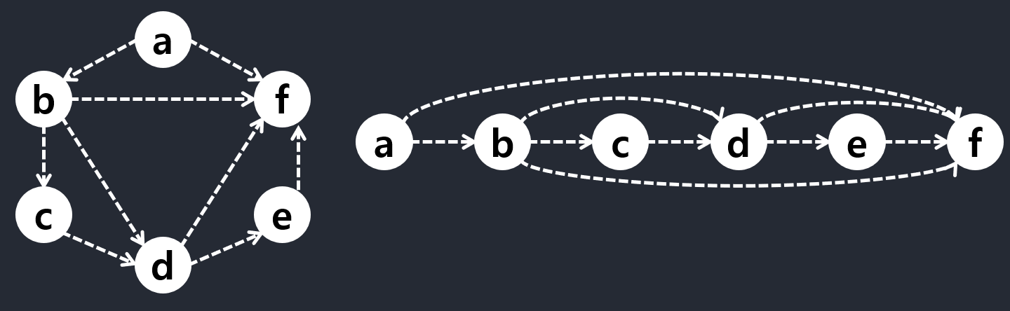
Figure 4-5 illustrates the concept. In this case, there is a unique valid ordering, but consider what would happen if you removed the edge ab, for example—then a could be placed anywhere in the order, as long as it was before f.

Most modern operating systems have at least one system for automatically installing software components (such as applications or libraries), and these systems can automatically detect when some dependency is missing and then download and install it. For this to work, the components must be installed in a topologically sorted order.

The next step is to look for some useful reduction. As before, our first intuition should probably be to remove a node and solve the problem (or assume that it is already solved) for the remaining n–1. This reasonably obvious reduction can be implemented in a manner similar to insertion sort.

def naive_topsort(G, S=None): 
    if S is None: S = set(G)                    # Default: All nodes 
    if len(S) == 1: return list(S)              # Base case, single node 

    v = S.pop()                                 # Reduction: Remove a node 
    seq = naive_topsort(G, S)                   # Recursion (assumption), n-1 
    min_i = 0 

    for i, u in enumerate(seq): 
        if v in G[u]: min_i = i+1               # After all dependencies 
    seq.insert(min_i, v) 

    return seq

Although I hope it’s clear (by induction) that naive_topsort is correct, it is also clearly quadratic. The problem is that it chooses an arbitrary node at each step, which means that it has to look where the node fits after the recursive call (which gives the linear work). We can turn this around and work more like selection sort. Find the right node to remove before the recursive call. This new idea, however, leaves us with two questions.
First, which node should we remove?
And second, how can we find it efficiently?

We’re working with a sequence (or at least we’re working toward a sequence), which should perhaps give us an idea. We can do something similar to what we do in selection sort and pick out the element that should be placed first.

Here, we can’t just place it first—we need to really remove it from the graph, so the rest is still a DAG (an equivalent but smaller problem). Luckily, we can do this without changing the graph representation directly, as you’ll see in a minute.

How would you find a node that can be put first? There could be more than one valid choice, but it doesn’t matter which one you take. I hope this reminds you of the maximum permutation problem. Once again, we want to find the nodes that have no in-edges. A node without in-edges can safely be placed first because it doesn’t depend on any others. If we (conceptually) remove all its out-edges, the remaining graph, with n–1 nodes, will also be a DAG that can be sorted in the same way.
Just like in the maximum permutation problem, we can find the nodes without in-edges by counting.

The only assumption about the graph representation is that we can iterate over the nodes and their neighbors.

Counting-based topological sorting:

def topsort(G): 
    count = dict((u, 0) for u in G)             # The in-degree for each node 

    for u in G: 
        for v in G[u]: 
            count[v] += 1                       # Count every in-edge 

    Q = [u for u in G if count[u] == 0]         # Valid initial nodes 
    S = []                                      # The result 

    while Q:                                    # While we have start nodes... 

        u = Q.pop()                             # Pick one 
        S.append(u)                             # Use it as first of the rest 

        for v in G[u]: 
            count[v] -= 1                       # "Uncount" its out-edges
            if count[v] == 0:                   # New valid start nodes? 
                Q.append(v)                     # Deal with them next 
    return S

reference:

Radix Sort: https://m.blog.naver.com/PostView.nhn?blogId=jhc9639&logNo=221258770067&proxyReferer=https:%2F%2Fwww.google.com%2F
Bucket Sort: https://ratsgo.github.io/data%20structure&algorithm/2017/10/18/bucketsort/