cs231n Assignment

July 2, 2021 10 minute read

1. 예제 따라하고, 개인 Github 정리하기

CNN

https://pytorch.org/tutorials/beginner/blitz/cifar10_tutorial.html#sphx-glr-beginner-blitz-cifar10-tutorial-py 사진 분류
https://pytorch.org/vision/stable/models.html 의 PyTorchVision을 참고하여 Pre-Trained AlexNet/VGG/ResNet/DenseNet 성능 비교하기
https://pytorch.org/tutorials/beginner/transfer_learning_tutorial.html 의 전이학습

RNN

https://pytorch.org/tutorials/intermediate/char_rnn_classification_tutorial.html# 의 이름 분류
https://pytorch.org/tutorials/beginner/text_sentiment_ngrams_tutorial.html 의 문자 분류
https://pytorch.org/tutorials/intermediate/seq2seq_translation_tutorial.html 의 번역
https://pytorch.org/tutorials/beginner/transformer_tutorial.html 의 TRANSFORMER 구조 번역

2. Multi-Layer Fully Connected Neural Networks

The notebook FullyConnectedNets.ipynb will have you implement fully connected networks of arbitrary depth. To optimize these models you will implement several popular update rules.

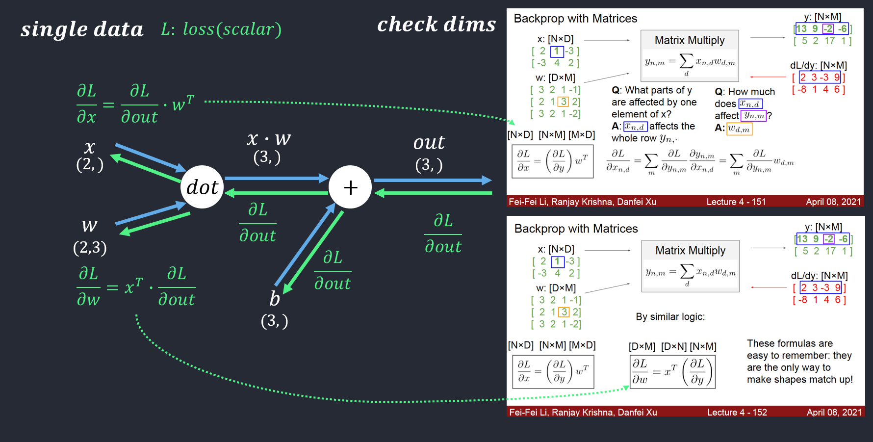
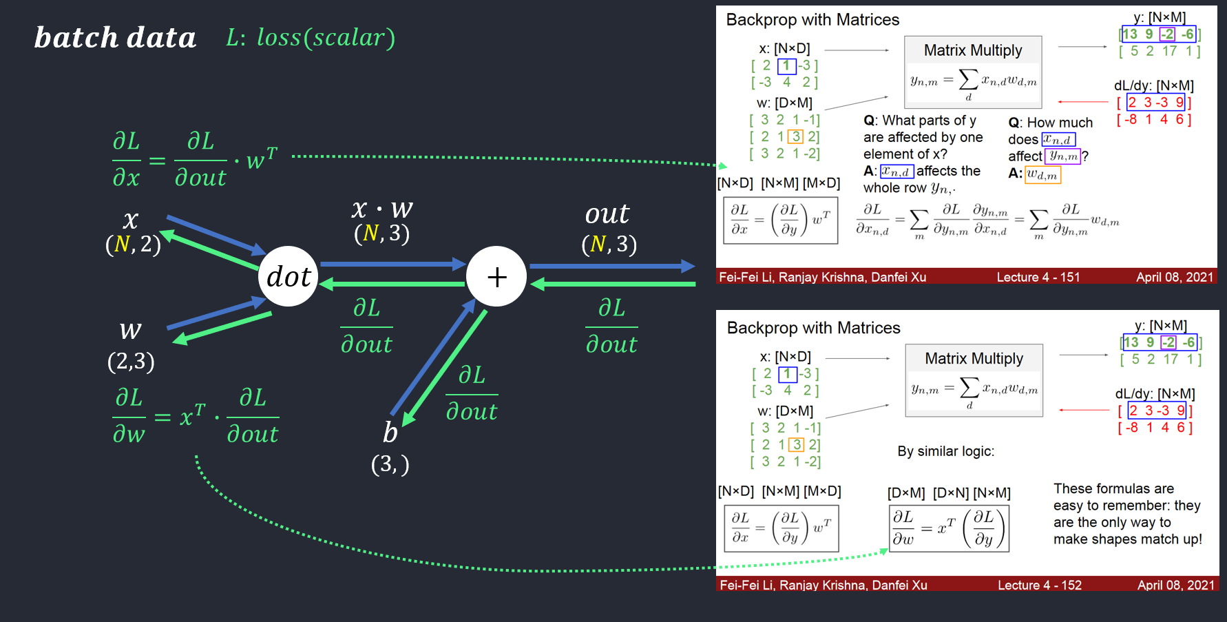
Affine Layer

Affine transform (dot Product):
Affine이라 함은 순전파에서 수행하는 행렬의 내적을 기하학에서 부르는 말로 Input 값과 Weight 값들을 행렬 곱하여 계산하고 거기에 편향(Bias)를 추가하여 출력값 Y를 최종적으로 반환

backprop-matrices-1

forward in code:

out = x.reshape(x.shape[0], -1)@w + b

backward in code:

dx = dout.dot(w.T).reshape(x.shape)
dw = x.reshape(x.shape[0], -1).T.dot(dout)
db = np.sum(dout, axis=0) # axis=0: column

description

"""
Inputs:
- dout: Upstream derivative, of shape (N, M)
- cache: Tuple of:
    - x: Input data, of shape (N, d_1, ... d_k)
    - w: Weights, of shape (D, M)
    - b: Biases, of shape (M,)

Returns a tuple of:
- dx: Gradient with respect to x, of shape (N, d1, ..., d_k)
- dw: Gradient with respect to w, of shape (D, M)
- db: Gradient with respect to b, of shape (M,)
"""

Check dims ❗❗

dx:
- dx = dout.dot(w.T).reshape(x.shape)
- dout: (10,5)
- w: (6,5)
- dout.dot(w.T): (10,6)
- dout.dot(w.T).reshape(x.shape): (10,2,3)
dw:
- dw = x.reshape(x.shape[0], -1).T.dot(dout)
- x.shape[0]: batch size (x.shape = (10,2,3))
- x.reshape(x.shape[0], -1): (10,6)
- dout: (10,5)
db:
- shape should be equal to the dout’s column(dout: (10,5)).
- thus, db = np.sum(dout, axis=0), sum by row-wise.
- np.sum(dout, axis=0): (5,)
dout = out in image.

ReLU activation (Rectifier Linear Unit)

forward:
For \(x > 0\) the output is \(x\), i.e. \(f(x) = \max(0,x)\) backward:
if \(x < 0\), output is \(0\). if \(x > 0\), output is \(1\).

forwrd in code:

out = np.maximum(x, 0)
# or
# out = x * (x > 0)

backward in code:

dout[x<0] = 0
dx = dout

Two-layer network

modify
cs231n/classifiers/fc_net.py:

class TwoLayerNet(object):
    def __init__(
        self,
        input_dim=3 * 32 * 32,
        hidden_dim=100,
        num_classes=10,
        weight_scale=1e-3,
        reg=0.0,
    ):
        self.params = {}
        self.reg = reg

        self.params["W1"] = np.random.normal(0.0, weight_scale, (input_dim, hidden_dim))
        self.params["W2"] = np.random.normal(0.0, weight_scale, (hidden_dim, num_classes))
        self.params["b1"] = np.zeros(hidden_dim, dtype=float)
        self.params["b2"] = np.zeros(num_classes, dtype=float)

    def loss(self, X, y=None):

        scores = None

        out1, cache1 = affine_relu_forward(X, self.params["W1"], self.params["b1"])
        out2, cache2 = affine_forward(out1, self.params["W2"], self.params["b2"])
        scores = out2

        if y is None:
            return scores

        loss, grads = 0, {}

        loss, dscores = softmax_loss(scores, y)
        dout1, grads["W2"], grads["b2"] = affine_backward(dscores, cache2)
        dX, grads["W1"], grads["b1"] = affine_relu_backward(dout1, cache1)

        for w in ["W2", "W1"]:
            if self.reg > 0:
                loss += 0.5 * self.reg * (self.params[w] ** 2).sum()
            grads[w] += self.reg * self.params[w]

        return loss, grads

Solver

Modify
cs231n/optim.py:

import numpy as np


def sgd(w, dw, config=None):

    if config is None: config = {}
    config.setdefault('learning_rate', 1e-2)

    w -= config['learning_rate'] * dw
    return w, config


def sgd_momentum(w, dw, config=None):

    if config is None: config = {}
    config.setdefault('learning_rate', 1e-2)
    config.setdefault('momentum', 0.9)
    v = config.get('velocity', np.zeros_like(w))

    next_w = None

    v = config['momentum'] * v - config['learning_rate'] * dw
    next_w = w + v

    config['velocity'] = v

    return next_w, config



def rmsprop(w, dw, config=None):

    if config is None: config = {}
    config.setdefault('learning_rate', 1e-2)
    config.setdefault('decay_rate', 0.99)
    config.setdefault('epsilon', 1e-8)
    config.setdefault('cache', np.zeros_like(w))

    next_w = None
 
    config['cache'] = config['decay_rate'] * config['cache'] + (1-config['decay_rate']) * (dw*dw)
    next_w = w - config['learning_rate'] * dw / np.sqrt(config['cache'] + config['epsilon'])

    return next_w, config


def adam(w, dw, config=None):

    if config is None: config = {}
    config.setdefault('learning_rate', 1e-3)
    config.setdefault('beta1', 0.9)
    config.setdefault('beta2', 0.999)
    config.setdefault('epsilon', 1e-8)
    config.setdefault('m', np.zeros_like(w))
    config.setdefault('v', np.zeros_like(w))
    config.setdefault('t', 0)

    next_w = None

    config['t'] += 1
    config['m'] = config['beta1'] * config['m'] + (1-config['beta1']) * dw
    mt = config['m'] / (1-config['beta1']**config['t'])
    config['v'] = config['beta2'] * config['v'] + (1-config['beta2']) * (dw*dw)
    vt = config['v'] / (1-config['beta2']**config['t'])
    next_w = w - config['learning_rate'] * mt / (np.sqrt(vt) + config['epsilon'])

    return next_w, config

Multilayer network

modify
cs231n/classifiers/fc_net.py:

class FullyConnectedNet(object):

    def __init__(self, hidden_dims, input_dim=3*32*32, num_classes=10,
                 dropout=0, use_batchnorm=False, reg=0.0,
                 weight_scale=1e-2, dtype=np.float32, seed=None):

        self.use_batchnorm = use_batchnorm
        self.use_dropout = dropout > 0
        self.reg = reg
        self.num_layers = 1 + len(hidden_dims)
        self.dtype = dtype
        self.params = {}

        self.params['W1'] = weight_scale * np.random.randn(input_dim, hidden_dims[0])
        self.params['b1'] = np.zeros(hidden_dims[0])
        if self.use_batchnorm:
            self.params['gamma1'] = np.ones(hidden_dims[0])
            self.params['beta1'] = np.zeros(hidden_dims[0])

        for i in range(2, self.num_layers):
            self.params['W'+repr(i)] = weight_scale * np.random.randn(hidden_dims[i-2], hidden_dims[i-1])
            self.params['b'+repr(i)] = np.zeros(hidden_dims[i-1])
            if self.use_batchnorm:
                self.params['gamma'+repr(i)] = np.ones(hidden_dims[i-1])
                self.params['beta'+repr(i)] = np.zeros(hidden_dims[i-1])

        self.params['W'+repr(self.num_layers)] = weight_scale * np.random.randn(hidden_dims[self.num_layers-2], num_classes)
        self.params['b'+repr(self.num_layers)] = np.zeros(num_classes)

        self.dropout_param = {}
        if self.use_dropout:
            self.dropout_param = {'mode': 'train', 'p': dropout}
            if seed is not None:
                self.dropout_param['seed'] = seed

        self.bn_params = []
        if self.use_batchnorm:
            self.bn_params = [{'mode': 'train'} for i in range(self.num_layers - 1)]

        # Cast all parameters to the correct datatype
        for k, v in self.params.items():
            self.params[k] = v.astype(dtype)

    def loss(self, X, y=None):

        X = X.astype(self.dtype)
        mode = 'test' if y is None else 'train'

        if self.use_dropout:
            self.dropout_param['mode'] = mode
        if self.use_batchnorm:
            for bn_param in self.bn_params:
                bn_param['mode'] = mode

        scores = None

        cache = {}
        dropout_cache = {}
        prev_hidden = X

        for i in range(1, self.num_layers):
            if self.use_batchnorm:
                prev_hidden, cache[i] = affine_bn_relu_forward(prev_hidden, self.params['W'+repr(i)], self.params['b'+repr(i)], 
                                                               self.params['gamma'+repr(i)], self.params['beta'+repr(i)], 
                                                               self.bn_params[i-1])
            else:
                prev_hidden, cache[i] = affine_relu_forward(prev_hidden, self.params['W'+repr(i)], self.params['b'+repr(i)])
            if self.use_dropout:
                prev_hidden, dropout_cache[i] = dropout_forward(prev_hidden, self.dropout_param)

        scores, cache[self.num_layers] = affine_forward(prev_hidden, self.params['W'+repr(self.num_layers)],
                                                        self.params['b'+repr(self.num_layers)])

        # If test mode return early
        if mode == 'test':
            return scores

        loss, grads = 0.0, {}

        loss, dscores = softmax_loss(scores, y)
        sum_squares_of_w = 0
        for i in range(1, self.num_layers+1):
            sum_squares_of_w += np.sum(self.params['W'+repr(i)]*self.params['W'+repr(i)])
        loss += 0.5 * self.reg * sum_squares_of_w

        dhidden, dW, db = affine_backward(dscores, cache[self.num_layers])
        dW += self.reg * self.params['W'+repr(self.num_layers)]
        grads['W'+repr(self.num_layers)] = dW
        grads['b'+repr(self.num_layers)] = db

        for i in list(reversed(range(1, self.num_layers))):
            if self.use_dropout:
                dhidden = dropout_backward(dhidden, dropout_cache[i])
            if self.use_batchnorm:
                dhidden, dW, db, dgamma, dbeta = affine_bn_relu_backward(dhidden, cache[i])
                grads['gamma'+repr(i)] = dgamma
                grads['beta'+repr(i)] = dbeta
            else:
                dhidden, dW, db = affine_relu_backward(dhidden, cache[i])
            dW += self.reg * self.params['W'+repr(i)]
            grads['W'+repr(i)] = dW
            grads['b'+repr(i)] = db

        return loss, grads

Optimizers

SGD(w momentum), RMSProp, Adam, AdaGrad

Questions

Inline Question 1:

We’ve only asked you to implement ReLU, but there are a number of different activation functions that one could use in neural networks, each with its pros and cons. In particular, an issue commonly seen with activation functions is getting zero (or close to zero) gradient flow during backpropagation. Which of the following activation functions have this problem? If you consider these functions in the one dimensional case, what types of input would lead to this behaviour?

Sigmoid
ReLU
Leaky ReLU

Answer:

Sigmoid
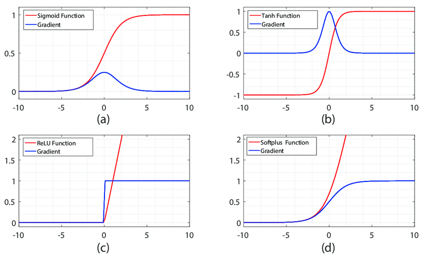
Sigmoid will appear positive and negative saturation, when the input value is very large or very small; ReLU will appear saturated in the negative half axis.

Inline Question 2(Weight Initialization):

Did you notice anything about the comparative difficulty of training the three-layer net vs training the five layer net? In particular, based on your experience, which network seemed more sensitive to the initialization scale? Why do you think that is the case?

Answer:

When training a 5-layer neural network with sgd before, I found that the weight initialization is particularly important: 1) The initialization is too small, which may cause the neurons of a certain layer to pass back; 2) the initialization is too large, which causes the occurrence of neurons in a certain layer Gradient explosion. Because weights are constantly involved in matrix multiplication, the deeper the network, the more important the weight initialization.

Weight Initialization (가중치 초기화)

학습의 성공 유무를 결정하는 중요한 요소
if 잘못된 가중치 초기화 ⇒ 역전파 알고리즘 진행간 아래와 같은 문제 발생 가능
- 1) vanishing gradient (그레디언트 소실)
- 2) exploding gradient (그레디언트 폭주)
  1) 초기값이 0 또는 같은 값으로 초기화한 경우
backpropation 진행 간 동일한 그래디언트로 가중치 값이 변경되기 때문에 뉴런의 개수가 많더라도
- ⇒ 결국, 뉴런이 하나인 경우와 동일하게 되어 학습이 제대로 이루어지지 않음 (시간만 더 소요될 듯)

2) 평균이 0이고 편차가 작은 난수로 초기화(일반적으로 평균 0, 표준편차 0.01인 가우시안 분포 사용)

얕은 신경망에서는 적용 가능 ⇒ but, 심층 신경망(DNN)에서는 적합하지 않음
- 출력 값이 모두 0이 되어 학습이 진행되지 않거나
- -1 또는 1로 집중되는 vanishing gradient 발생
  -위 문제점들을 해결하기 위해서는 뉴런의 활성화 함수 출력 값이 고르게 분포되어야 함

3) Xavier 초기화

tanh에 Xavier 초기화 방법을 적용한 결과 2)와 같이 작은 난수로 초기화한 경우보다 더 고른 분포를 보임

4) He 초기화

3)에서와 같이 Xavier 초기값은 tanh 활성화 함수에서는 좋은 결과를 보여주지만, ReLU 활성화 함수에서는
- layer가 깊어질수록 출력값이 0에 가까워지는 문제점이 발생
  Summary
Sigmoid ⇒ Xavier 초기화를 사용하는 것이 유리
ReLU ⇒ He 초기화 사용하는 것이 유리
- 활성화 함수는 기본적으로 ReLU 먼저 적용하는 것을 추천

Inline Question 3:

AdaGrad, like Adam, is a per-parameter optimization method that uses the following update rule:

cache += dw**2
w += - learning_rate * dw / (np.sqrt(cache) + eps)

John notices that when he was training a network with AdaGrad that the updates became very small, and that his network was learning slowly. Using your knowledge of the AdaGrad update rule, why do you think the updates would become very small? Would Adam have the same issue?

Answer:

The momentum of AdaGrad will not diminish over time. When the accumulated momentum gets larger and larger, the update step will become smaller and smaller, so a decay factor is required. And Adam will not have this problem.

3. Batch Normalization

In notebook BatchNormalization.ipynb you will implement batch normalization, and use it to train deep fully connected networks.
[Batch-Normalization-paper]https://arxiv.org/abs/1502.03167

Batch Normalization(배치 정규화)

각 층의 출력값들을 정규화하는 방법
Weight Initialization(가중치 초기화)와 더불어 학습의 성공 유무를 결정하는 중요한 요소
- 학습할 때마다 출력값을 정규화시키기 때문에 Weight Initialization(가중치 초기화)에 대한 의존도를 낮춤
vanishing gradient(그레디언트 소실)과 exploding gradient(그레디언트 폭주) 해결 ⇒ 보다 근본적인 방법
- ⇒ Learning rate(학습속도)를 크게 설정하는 것이 가능해져 학습속도가 빨라지고, overfitting 위험이 감소됨
심층 신경망일수록 가중치에 따라 input 값이 같더라도 output 값이 달라지게 되는 문제 발생
Batch normalization을 통한 출력값 정규화를 통해 이러한 차이를 줄여 안정적인 학습이 가능하게 할 수 있음
- 출력값 정규화에 필요한 parameter들은 backpropagation을 통해 학습 가능
입력 데이터(xi)를 정규화시키면 0에 가까운 값이 나오는데, 이러한 경우 signoid 함수 적용 시 문제점 발생
- ⇒ 이를 해결하기 위해 gamma(scale)과 Beta(shift)를 적용하여 yi 값을 계산함
  - gamma(scale)는 가중치(weight), Beta(shift)는 편항(bias)으로 볼 수 있으며, 각 1과 0으로 시작하여 역잔파를 통해 적합한 값으로 fitthing 됨
텐서플로에서는 tf.nn.batch_normalization과 tf.layers.batch_normalization 두개의 방법 제공
- parameter를 모두 계산해 주는 tf.layers.batch_normalization 추천

Batch normalization and initialization

Inline Question 1:

Describe the results of this experiment. How does the scale of weight initialization affect models with/without batch normalization differently, and why?

Answer:

Batch normalization and batch size

Inline Question 2:

Describe the results of this experiment. What does this imply about the relationship between batch normalization and batch size? Why is this relationship observed?

Answer:

Layer Normalization

[Layer-Normalization]https://arxiv.org/pdf/1607.06450.pdf

Inline Question 3:

Which of these data preprocessing steps is analogous to batch normalization, and which is analogous to layer normalization?

Scaling each image in the dataset, so that the RGB channels for each row of pixels within an image sums up to 1.
Scaling each image in the dataset, so that the RGB channels for all pixels within an image sums up to 1.
Subtracting the mean image of the dataset from each image in the dataset.
Setting all RGB values to either 0 or 1 depending on a given threshold.

Answer:

Layer Normalization and batch size

Inline Question 4:

When is layer normalization likely to not work well, and why?

Using it in a very deep network
Having a very small dimension of features
Having a high regularization term

Answer:

4. Convolutional Neural Networks

In the notebook ConvolutionalNetworks.ipynb you will implement several new layers that are commonly used in convolutional networks.

5. Image Captioning with Vanilla RNNs

The notebook RNN_Captioning.ipynb will walk you through the implementation of vanilla recurrent neural networks and apply them to image captioning on COCO.

One advantage of an image-captioning model that uses a character-level RNN is that they have a very small vocabulary. For instance, let’s suppose we have a dataset with one million of different words. If we use the word-level model then it will require more memory than the character-level model because the number of characters used to represent all of the words will be smaller.

One disadvantage is that the number of parameters will increase because we have a larger sequence. In the aforementioned example, the number of hidden layers will be equal to the number of characters (10 layers without considering the space character). On the other hand by using the word-level model, the number of hidden layers will be equal to 5. Having a small number of parameters is computationally more efficient and less prone to vanishing/exploding gradients.

Appendix

References

Affine transform: https://ayoteralab.tistory.com/entry/ANN-11-%ED%99%9C%EC%84%B1%ED%99%94%ED%95%A8%EC%88%98s-Back-Propagation-Affine-Softmax
Affine transform: https://sacko.tistory.com/39
explanation: https://m.blog.naver.com/PostView.naver?isHttpsRedirect=true&blogId=tinz6461&logNo=221583992917
https://www.programmersought.com/article/80444944178/
Weight Initialization: https://m.blog.naver.com/tinz6461/221599717016
Batch Normalization: https://m.blog.naver.com/tinz6461/221599876015 Batch Normalization & Weight Initialization: https://www.programmersought.com/article/22581368882/
BN: https://www.programmersought.com/article/3460593295/

Share on

Twitter Facebook LinkedIn

Yilguk Seo 🚀

1. 예제 따라하고, 개인 Github 정리하기

CNN

RNN

2. Multi-Layer Fully Connected Neural Networks

Affine Layer

ReLU activation (Rectifier Linear Unit)

Two-layer network

Solver

Multilayer network

Optimizers

SGD(w momentum), RMSProp, Adam, AdaGrad

Questions

Inline Question 1:

Answer:

Inline Question 2(Weight Initialization):

Answer:

Weight Initialization (가중치 초기화)

1) 초기값이 0 또는 같은 값으로 초기화한 경우

2) 평균이 0이고 편차가 작은 난수로 초기화(일반적으로 평균 0, 표준편차 0.01인 가우시안 분포 사용)

3) Xavier 초기화​

4) He 초기화

Summary

Inline Question 3:

Answer:

3. Batch Normalization

Batch Normalization(배치 정규화) ​

Batch normalization and initialization

Inline Question 1:

Answer:

Batch normalization and batch size

Inline Question 2:

Answer:

Layer Normalization

Inline Question 3:

Answer:

Layer Normalization and batch size

Inline Question 4:

Answer:

4. Convolutional Neural Networks

5. Image Captioning with Vanilla RNNs

Appendix

References

Share on

Leave a comment

You may also enjoy

시작

ML Flow Tutorial

Windows gitlab ssh

Git bash & conda in Windows

3) Xavier 초기화

Batch Normalization(배치 정규화)