NN basics - DL Optimization

Objective Function

Objective Funtion Vs. Loss Function(alias: Cost Function)

“The function we want to minimize or maximize is called the objective function, or criterion. When we are minimizing it, we may also call it the cost function, loss function, or error function. In this book, we use these terms interchangeably, though some machine learning publications assign special meaning to some of these terms.” (“Deep Learning” - Ian Goodfellow, Yoshua Bengio, Aaron Courville)
Loss function is usually a function defined on a data point.

MSE

\(e = \frac{1}{2}\Vert \boldsymbol{y} - \boldsymbol{o}\Vert_{2}^{2}\)

오차가 클 수록 \(e\) 값이 크므로 벌점으로 활용됨

MSE bad for NN(with sigmoid)

• 신경망 학습과정에서 학습은 오류를 줄이는 방향으로 가중치와 편향을 교정하는데 큰 교정이 필요함에도 gradient가 작게 갱신됨.
  -이유: error가 커져도 logistic sigmoid의 gradient는 값이 커질수록 vanishing되기 때문.
• good for linear regression

What if NN uses other activation function except sigmoid or tanh? Still considered as useful or not?

CrossEntropy

확률분포의 차이를 비교하는 함수

Softmax & Negtative Log Likelihood (NLL)

Softmax:
모두 더하면 1이 되기 때문에 확률을 모방.

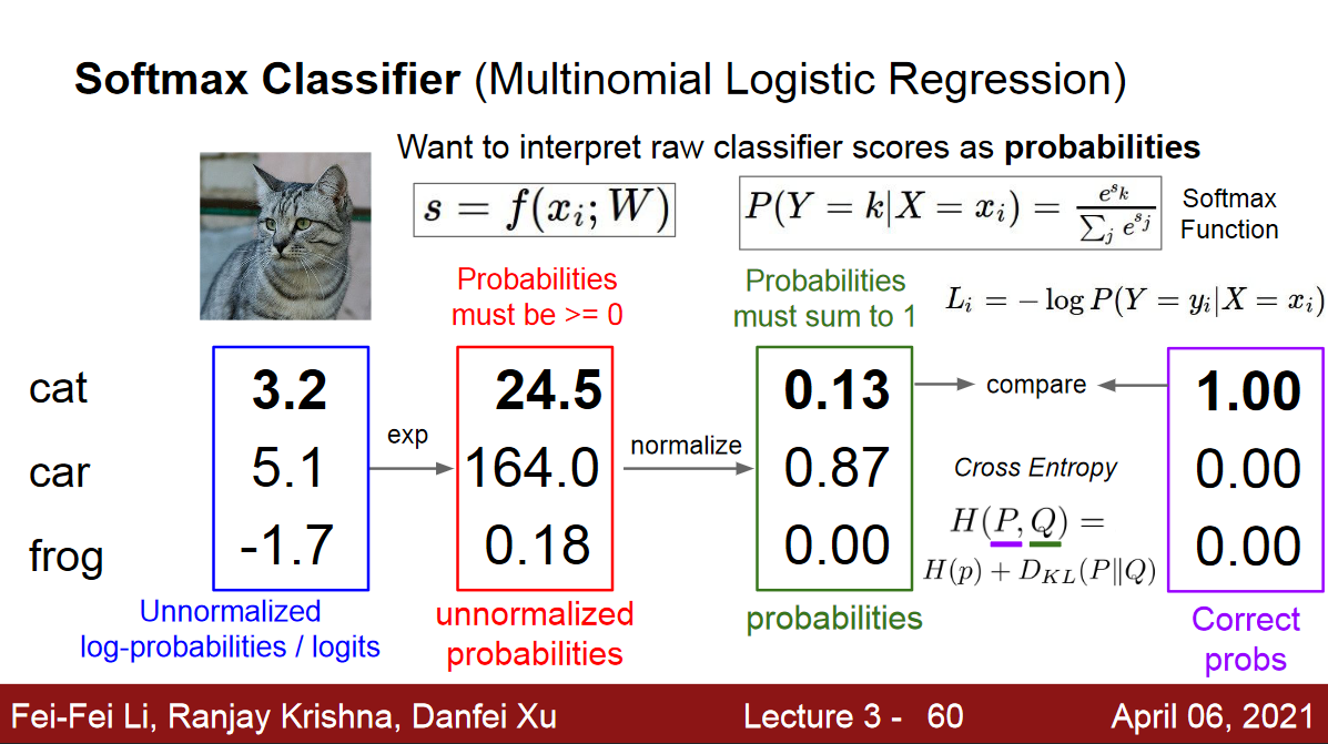
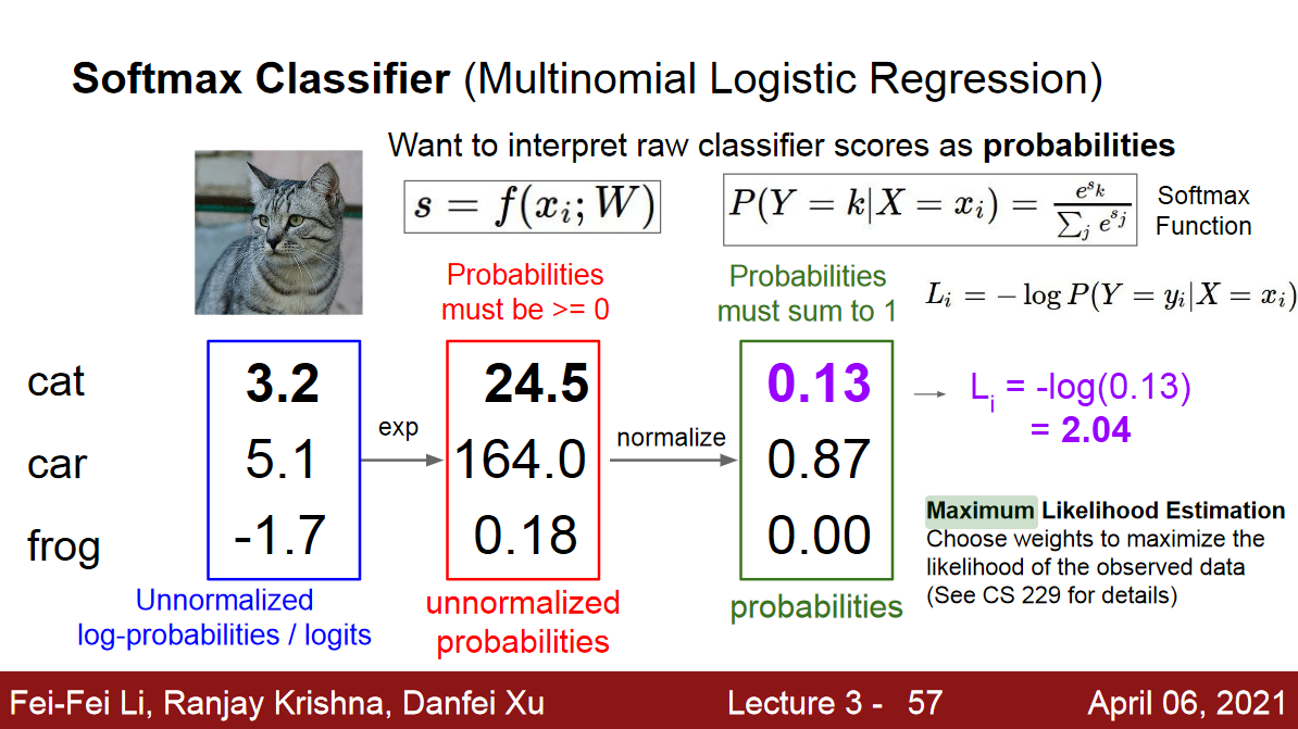
NLL의 경우 target값의 index와 예측값의 index만을 사용

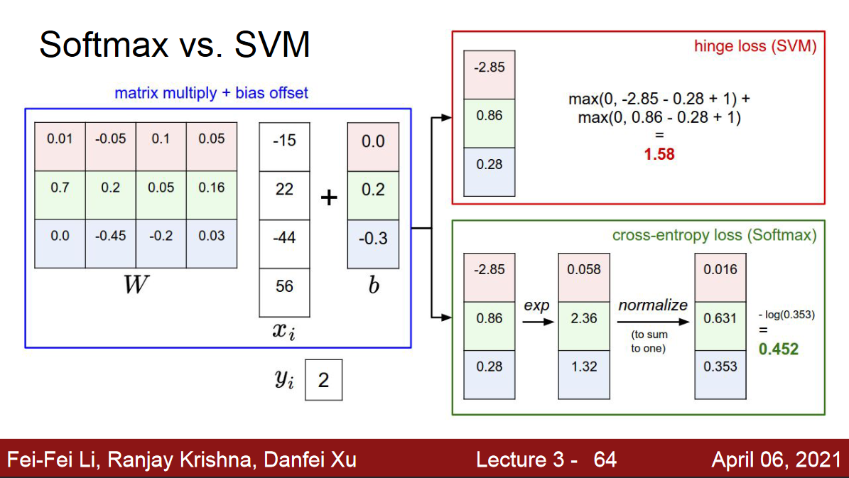
Softmax Vs. Hinge Loss

Pre-Processing

Normalization

• 특징값이 모두 양수(또는 모두 음수)이거나 특징마다 값의 규모가 다르면, 수렴 속도가 느려질 수 있다.
  • 모든 x가 양인 상황에서 어떤 오차역전파 σ값은 음수인 상황에는 양의 방향으로 업데이트 되지만, σ값이 양수인 상황에서는 음의 방향으로 업데이트 된다. 이처럼 여러 가중치가 뭉치로 같이 증가하거나, 감소하면 최저점을 찾아가는 경로를 갈팡질팡하여 수렴 속도 저하로 이어진다.
• 또한 특징의 규모가 달라 (예를 들어, 1.75m 등의 값을 가지는 키 특징과, 60kg 등의 값을 가지는 몸무게 특징은 스케일이 다르다) 특징마다 학습속도가 다를 수 있으므로, 전체적인 학습 속도는 저하될 것이다.

특징별로 독립적으로 적용.

• 정규분포를 활용해서 Normalization.
• Max & Min Scaler

One Hot Encoding

Weight Initialization

Symmetric Weight

When some machine learning models have weights all initialized to the same value, it can be difficult or impossible for the weights to differ as the model is trained. This is the “symmetry”. Initializing the model to small random values breaks the symmetry and allows different weights to learn independently of each other.
같은 값으로 가중치를 초기화 시키면, 두 노드가 같은 일을 하게 되는 중복성 문제가 생길 수 있다. 따라서 이런 일을 피하는 대칭 파괴(Symmetry break)가 필요하다.

Random Initialization

난수는 가우시안분포(Gaussian Distribution 또는 균일 분포(Uniform Distribution) 추출할 수 있고, 실험 결과 둘의 차이는 별로 없다고 함.

바이어스는 보통 0으로 초기화 한다.

중요한 것은 난수의 범위인데, 극단적으로 가중치가 0에 가깝게 되면 그레디언트가 아주 작아져 학습이 느려지고, 반대로 너무 크면 과잉적합의 위험이 있다.

Visualization

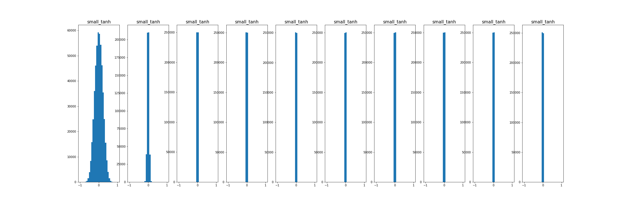
• 초기화가 너무 작으면, 모든 활성 값이 0이 됨. 경사도도 역시 영. 학습 안됨

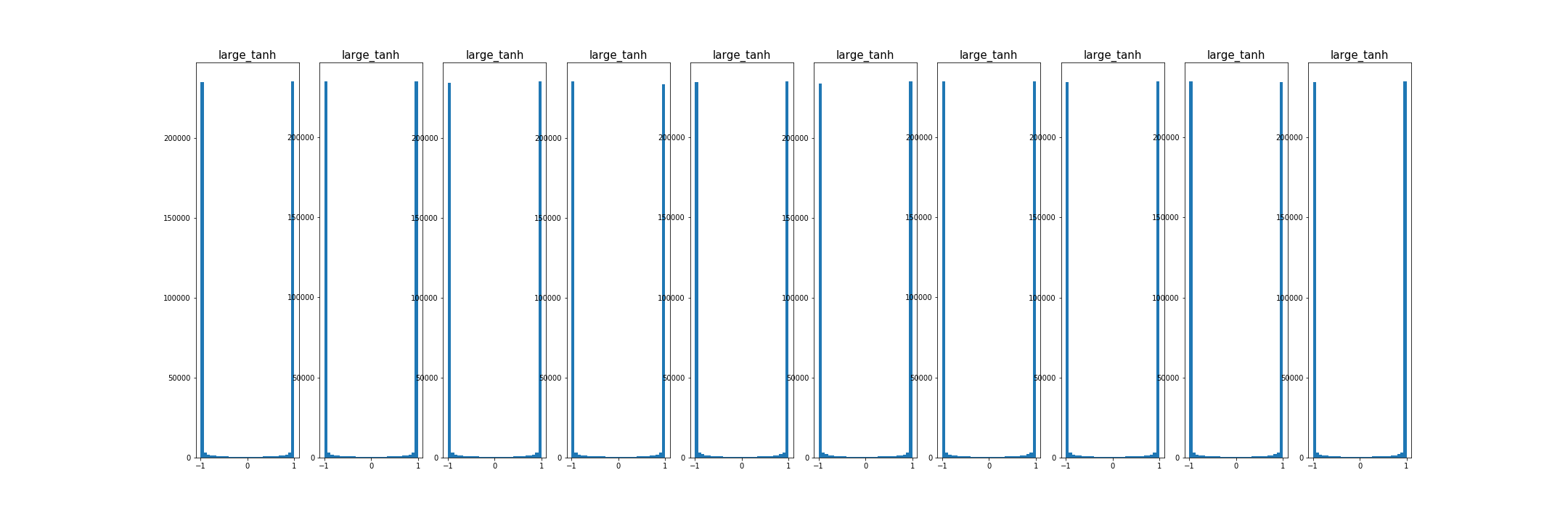
• 초기화가 너무 크면, 활성값 포화, 경사도 0, 학습안됨.

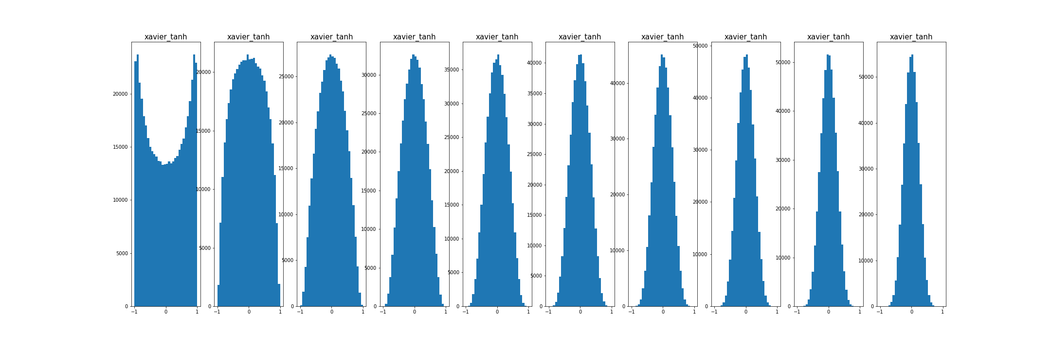
• 초기화가 적당하다면, 모든 층에서 활성 값의 분포가 좋음.

추가적으로,

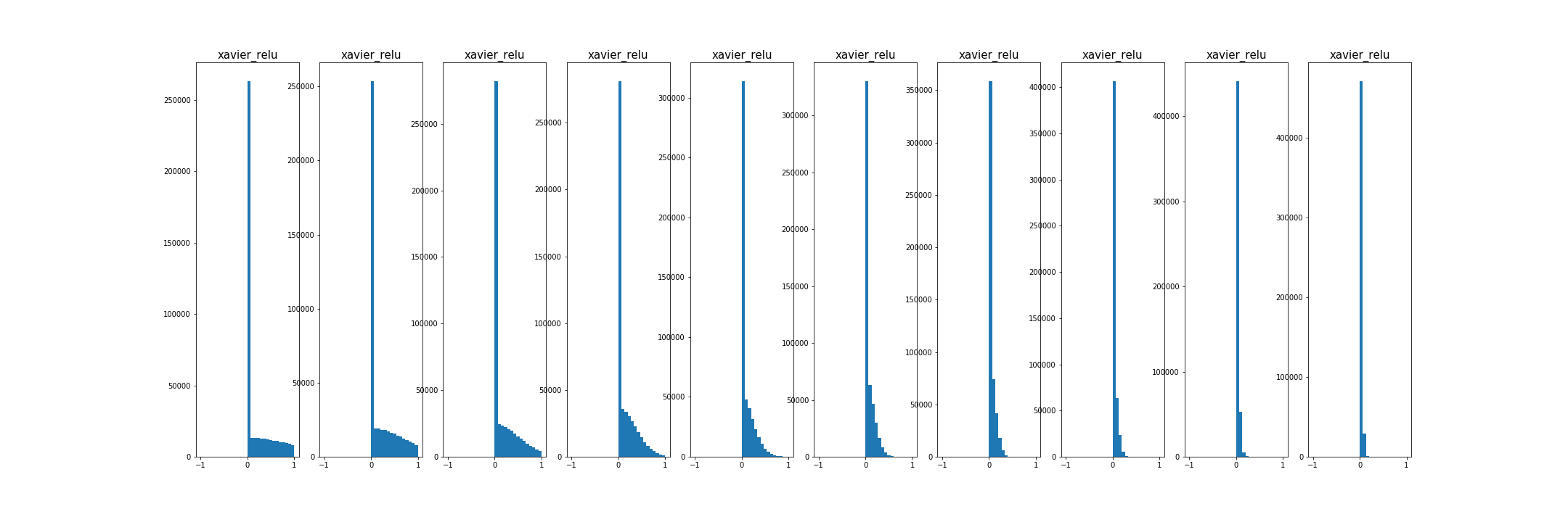
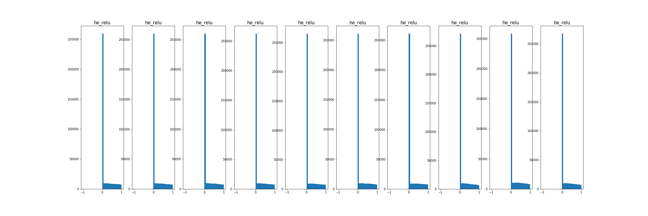
• conclusion on Weight Initialization
  • sigmoid, tanh : Xavier
  • ReLU : He

Weight initialization visualization code:

import numpy as np
from matplotlib.pylab import plt

# assume some unit gaussian 10-D input data
def weight_init(types, activation):
    D = np.random.randn(1000, 500)
    hidden_layer_sizes = [500]*10
    if activation == "relu":
        nonlinearities = ['relu']*len(hidden_layer_sizes)
    else:
        nonlinearities = ['tanh']*len(hidden_layer_sizes)

    act = {'relu': lambda x:np.maximum(0,x), 'tanh':lambda x: np.tanh(x)}
    Hs = {}

    for i in range(len(hidden_layer_sizes)):
        X = D if i==0 else Hs[i-1] # input at this layer
        fan_in = X.shape[1]
        fan_out = hidden_layer_sizes[i]
        if types == "small":
            W = np.random.randn(fan_in, fan_out) * 0.01 # layer initialization
        elif types == "large":
            W = np.random.randn(fan_in, fan_out) * 1 # layer initialization
        elif types == "xavier":
            W = np.random.randn(fan_in, fan_out) / np.sqrt(fan_in) # layer initialization
        elif types == "he":
            W = np.random.randn(fan_in, fan_out) / np.sqrt(fan_in/2) # layer initialization
            

        H = np.dot(X, W) # matrix multiply
        H = act[nonlinearities[i]](H) # nonlinearity
        Hs[i] = H # cache result on this layer

    print('input layer had mean', np.mean(D), 'and std', np.std(D))

    # look at distributions at each layer
    layer_means = [np.mean(H) for i,H in Hs.items()]
    layer_stds = [np.std(H) for i,H in Hs.items()]

    # print
    for i,H in Hs.items() :
        print('hidden layer', i+1, 'had mean', layer_means[i], 'and std', layer_stds[i])

    plt.figure();
    plt.subplot(1,2,1);
    plt.title("layer mean");
    plt.plot(range(10), layer_means, 'ob-');
    plt.subplot(1,2,2);
    plt.title("layer std");
    plt.plot(range(10), layer_stds, 'or-');

    plt.show();

    plt.figure(figsize=(30,10));
    
    for i,H in Hs.items() :
        
        plt.subplot(1,len(Hs), i+1)
        plt.hist(H.ravel(), 30, range=(-1,1))
    plt.title("{}_{}".format(types, activation), fontsize = 15)
    plt.show();
    save_path = "images/{}_{}.png".format(types, activation)
    print("saved at : {}".format(save_path))
    plt.savefig(save_path);

weight_init('xavier', 'tanh') # small, large, xavier, he; tanh, relu

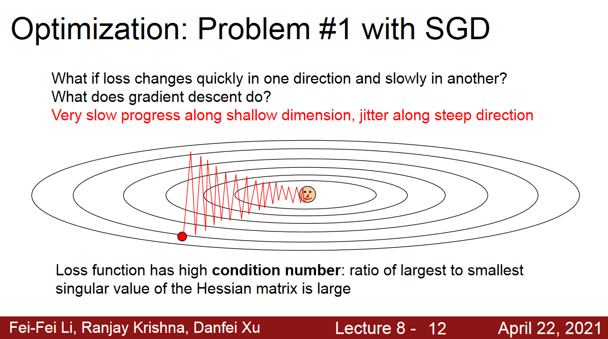
Momentum (Problem with SGD)

과거에 이동했던 방식을 기억하면서 기존 방향으로 일정 이상 추가 이동함.
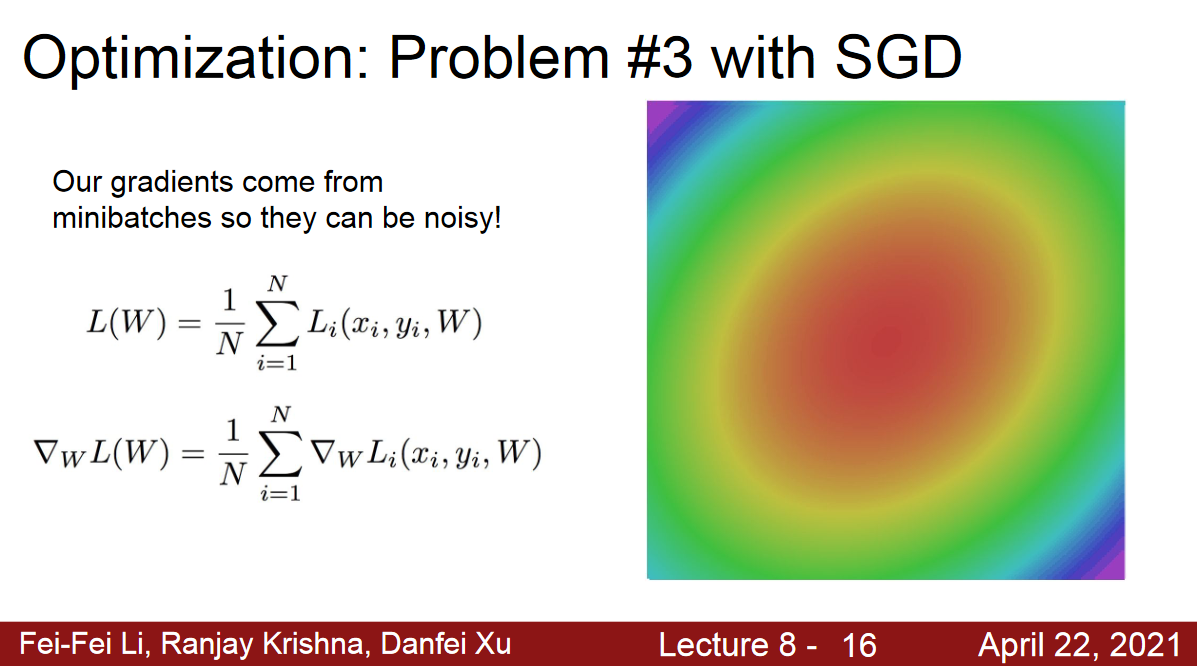
Gradient Noise를 해결하기 위함.

• \(\rho\) 가 momentum을 결정하는 것임. \(\rho = 0\)이면 모멘텀이 없는 것. 속도를 더하는 것(cs231에서는 friction이라고 표현함 마찰을 줄임).

  Jitter along steep direction

  

  local minima or saddle point

  

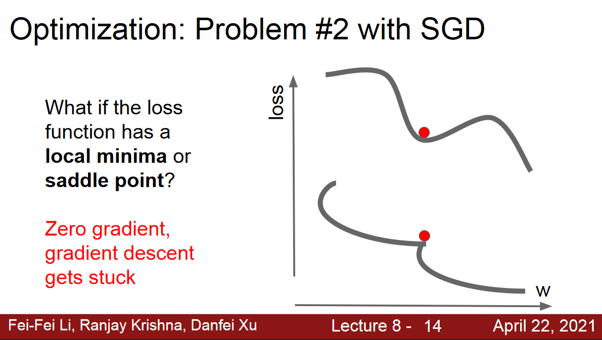
• Saddle points much more common in high dimension.

  Minibatch could be more noisy

  

Nesterov Momentum

원래 SGD:
gradient 구하고 momentum 더해서 이동

Nesterov Momentum:
momentum 더한후 gradient 구하고 이동

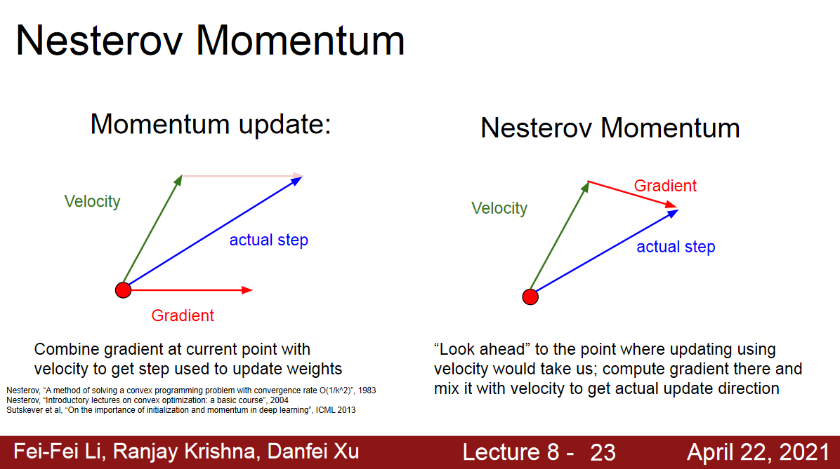
If your velocity was actually a little bit wrong, it lets you incorporate gradient information from a little bit larger parts of the objective landscape. (momentum이 주는 속도가 틀렸을 경우 최적의 landscape, 여기서는 loss가 optimal minima로 향하는 곳인듯,에 꽤나 큰 정보를 제공한다는 의미인듯.).

Adaptive Learning Rates

이전 경사도와 현재 경사도의 부호가 같은 경우 값을 키우고 다른 경우 값을 줄이는 전략

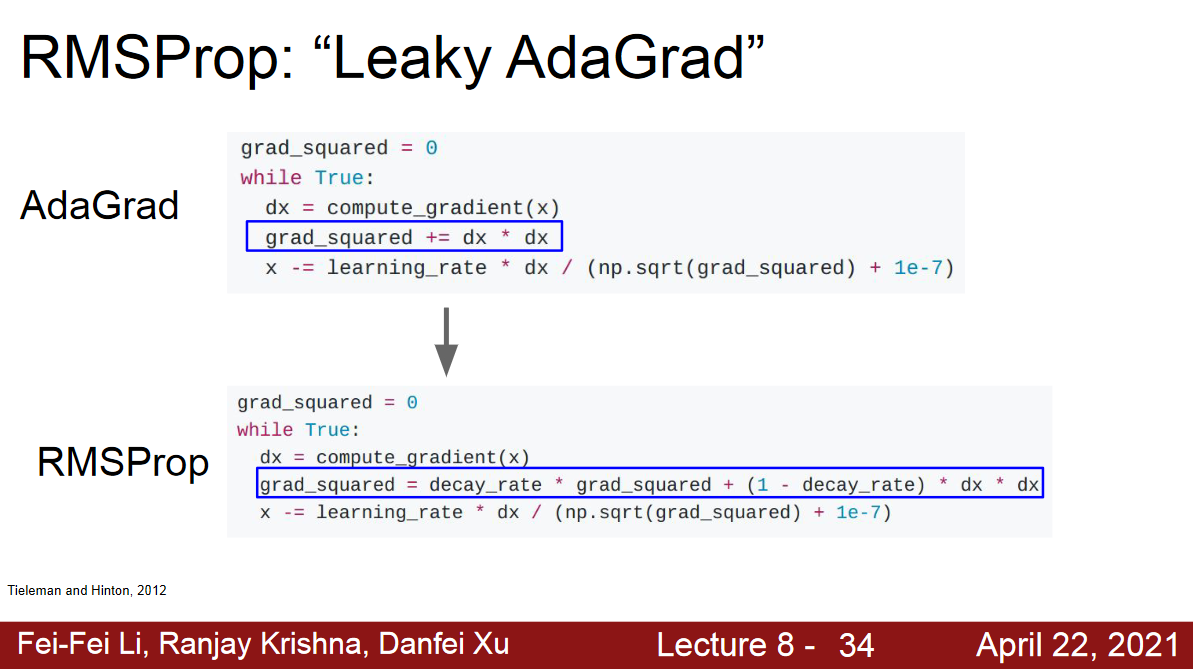
AdaGrad(Adaptive Gradient)

속도 대신에 squared term을 사용함.

두 개의 coordinate가 있다고 했을때, 한 쪽은 high gradient, 반대쪽은 small gradient, sum of squares of the small gradient 하고 small gradient으로 나눈다면,
accelerate the movement along the long dimension. Then, along the other dimension, where the gradients tend to be very large, then we’ll be dividing by a large number, so slow down the progress.

• 지난 경사도와 최근 경사도는 같은 비중
  • \(r\)이 점점 커져 수렴을 방해할 가능성.
  • convex case, slow down and converge
  • non-convex case, can be stuck in saddle point making no longer progress

RMSProp (variation of AdaGrad)

WMA(weighted moving average): 최근 것에 비중을 둠.

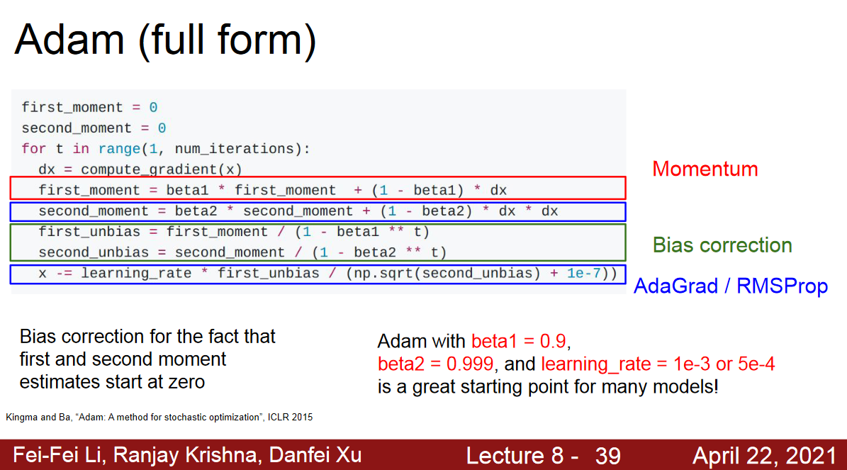
Adam (Adaptive Moment Estimation: RMSProp with momentum)

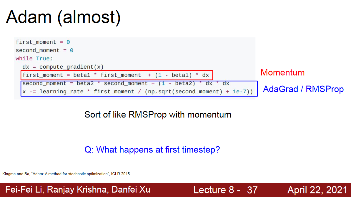
Q: What happens at first timestep?

At the very first timestep, you can see that at the beginning, we’ve initialized second_moment with zero. After one update of the second_moment, typically beta2, second_moment’s decay rate, is something like 0.9 or 0.99 something very close to 1. So after one update, our second_moment is still very close to zero. When we’re making update step, and divide by our second_moment, now we’re dividing by very small number. So, we’re making a very large step at the beginning. This very large step at the beginnig is not really due to the geometry of the problem. It’s kind of an artifact of the fact that we initialized our second_moment estimate was zero.

---

Q: If your first moment is also very small, then you’re multiplying by small and dividing by square root of small squared, what’s going to happen?

They might cancel each other out and this might be okay. Sometimes these cancel each other out. But, sometimes this ends up in taking very large steps right at the beginning. That can be quite bad. Maybe you initialize a little bit poorly, and you take a very large step. Now your initialization is completely messed up, and you’re in a very bad part of the objective landscape and you just can’t converge there.

---

Bias correction term:

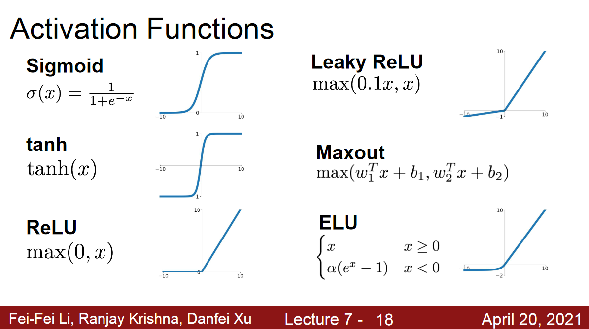
Activation Function

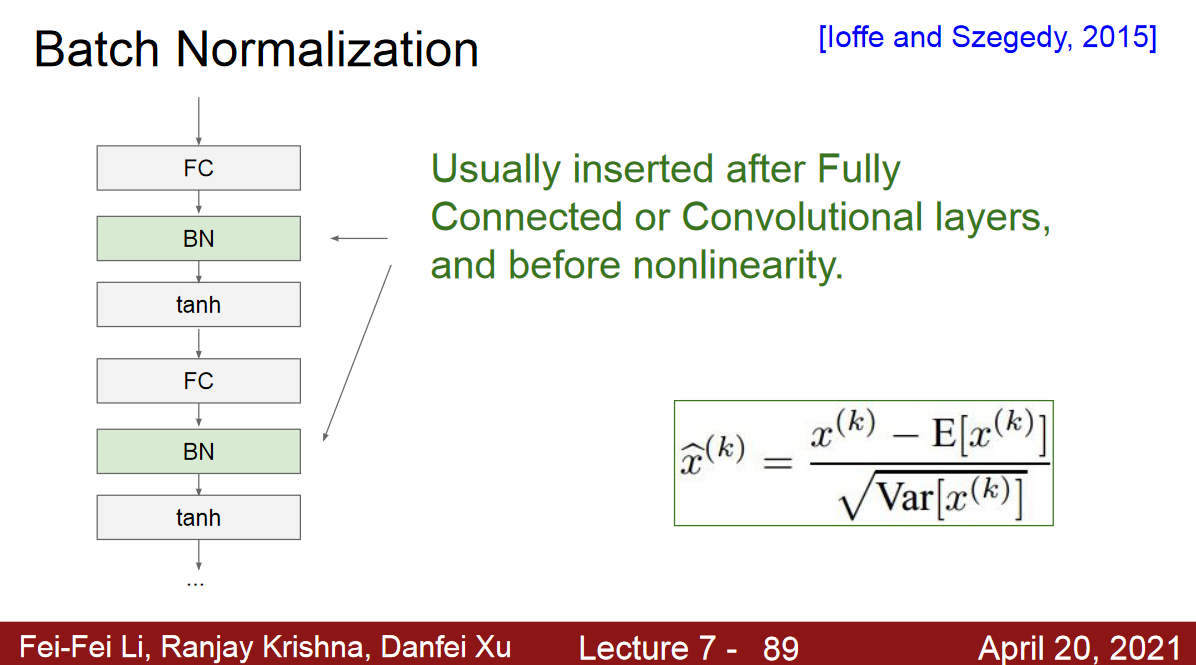
Batch Normalization

Covariate Shift: train set, test set의 분포가 다름.
Internal Covariate Shift: 학습이 진행되면서 다음 층에서는 데이터의 분포가 수시로 바뀌기 때문에 학습에 방해가 될 수 있음.

정규화를 층 단위 적용하는 기법

층은 선형적 연산과 비선형적 연산으로 구성되는 데,
여기서에서 어디에 정규화를 적용할 것인가?

• 선형 연산 후에 바로 정규화를 적용(즉, activation 전에)
• 일반적으로 fc, conv 후 또는 activation 전에 적용

미니배치에 적용하는 것이 유리.

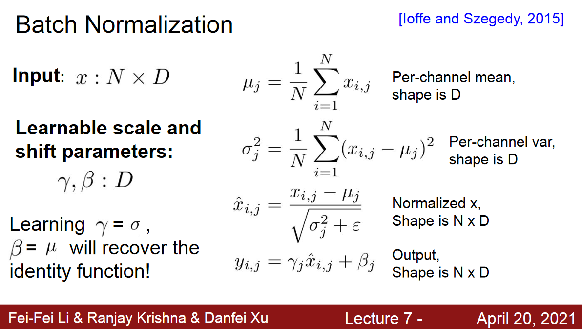
BN Process

1. 미니 배치로 평균과 분산 계산 (\(\mu, \sigma\))
2. \(\mu, \sigma\)를 통해 정규화
3. 비례(scale)와 이동(shift) 으로 세부 조정 (\(\gamma, \beta\), 이 둘도 학습에 의해 결정됨)
   • Maybe in particular part of the network gives flexibility in normalization.

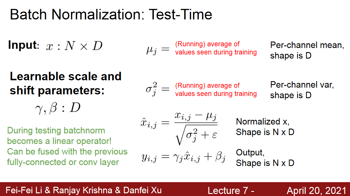
BN inference

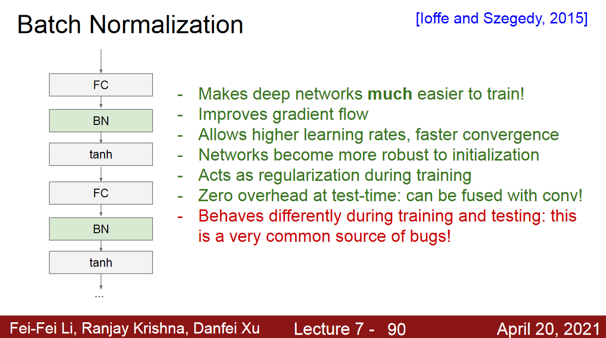
Advantages

• Gradient 개선
• Large LR 허용
• 초기화 의존성 감소
• 규제화 효과로 dropout 필요성 감소.

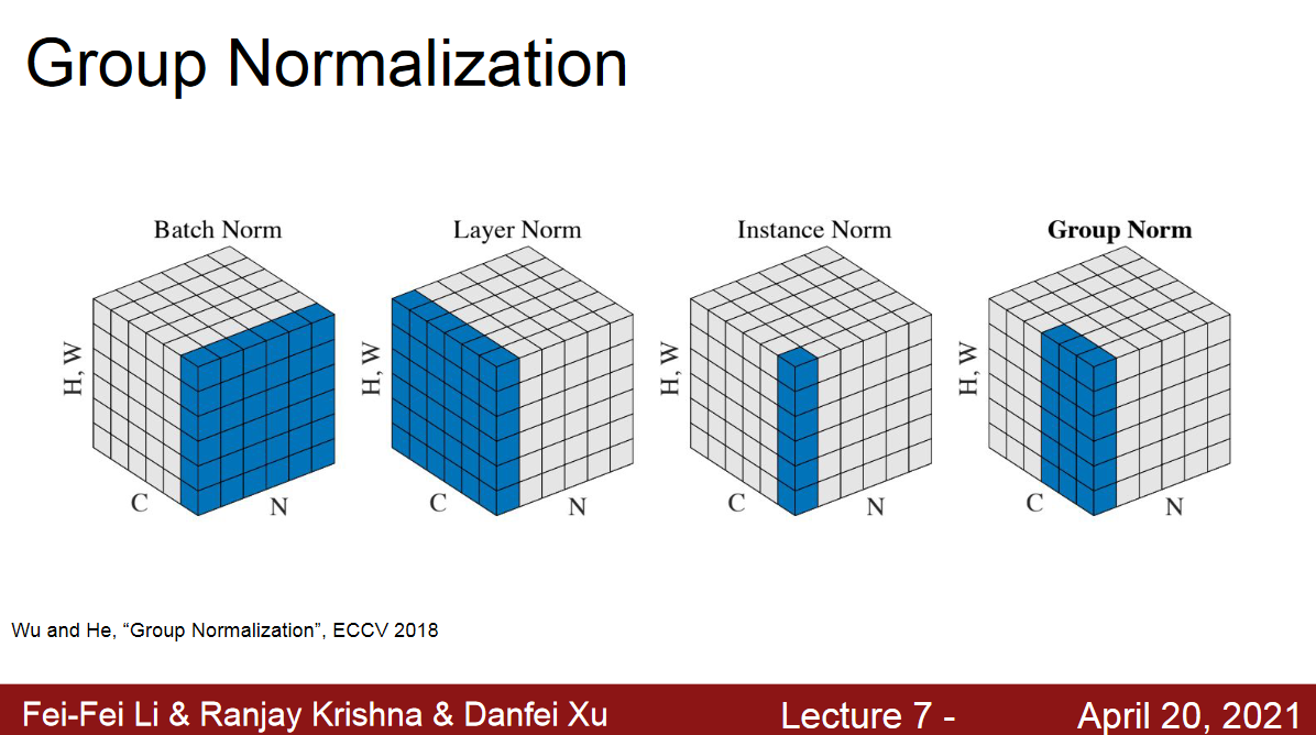
Types of Normalizations

Regularization

Methods

Add extra Term to Loss

• Regularization term은 훈련집합과 무관, 데이터 생성 과정에 내재한 사전 지식에 해당.
• 파라미터를 작은 값으로 유지하므로 모델의 용량을 제한하기도 함.
• 작은 가중치를 유지하려고 l2 norm, l1 norm을 주로 사용

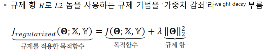
  L2 Norm

Early Stopping

Data Augmentation

Drop Out

fc에서 발생하는 overfitting을 줄이기 위해서 씀.

Co-Adaptation

데이터의 각각의 network의 weight들이 서로 동조화 되는 현상이 발생(신경망 구조의 inherent한 특성).
random하게 dropout을 주면서 이러한 현상을 규제하는 효과.

In a standard neural network, the derivative received by each parameter tells it how itshould change so the final loss function is reduced, given what all other units are doing.Therefore, units may change in a way that they fix up the mistakes of the other units.This may lead to complex co-adaptations. This in turn leads to overfitting because these co-adaptations do not generalize to unseen data. We hypothesize that for each hidden unit, dropout prevents co-adaptation by making the presence of other hidden units unreliable.Therefore, a hidden unit cannot rely on other specific units to correct its mistakes. It mustperform well in a wide variety of different contexts provided by the other hidden units. paper

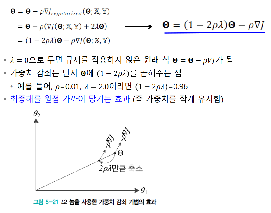
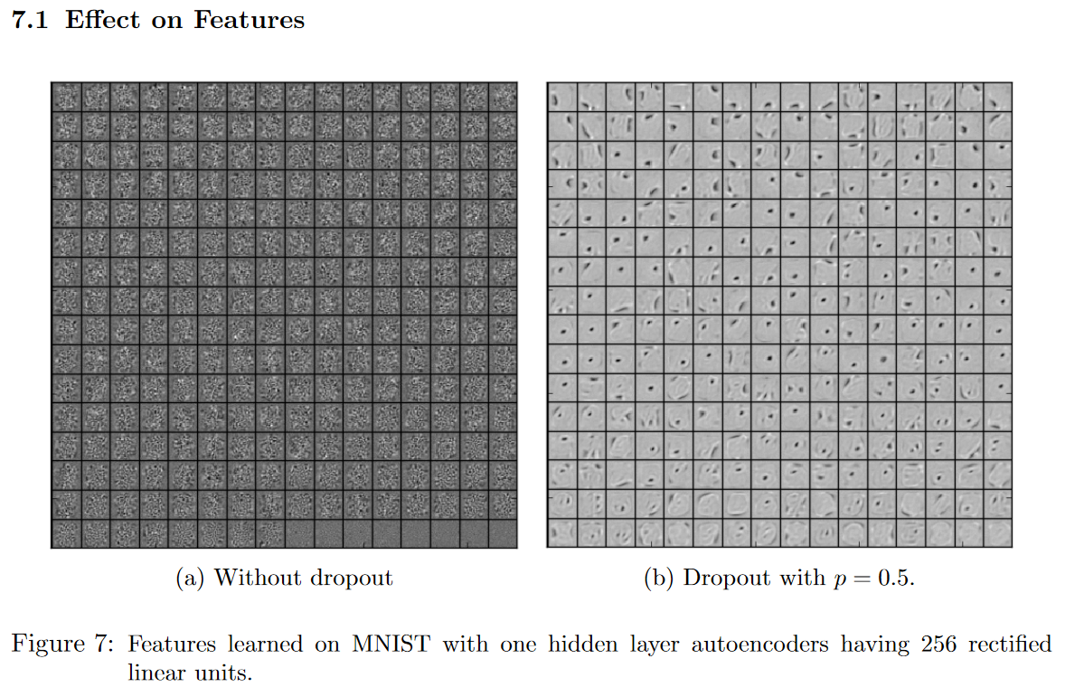
Figure 7a shows features learned by an autoencoder on MNIST with a single hiddenlayer of 256 rectified linear units without dropout. Figure 7b shows the features learned byan identical autoencoder which used dropout in the hidden layer withp= 0.5. Both au-toencoders had similar test reconstruction errors. However, it is apparent that the featuresshown in Figure 7a have co-adapted in order to produce good reconstructions. Each hiddenunit on its own does not seem to be detecting a meaningful feature. On the other hand, inFigure 7b, the hidden units seem to detect edges, strokes and spots in different parts of theimage. This shows that dropout does break up co-adaptations, which is probably the mainreason why it leads to lower generalization errors.

Sparsity

hidden 뉴런들의 활성도가 좀 더 sparse 됨.
sparse하게 되면서 의미가 있는 부분만 더 남게 되는 효과를 가지게 되는 것임(sparse하지 않고 골고루 분포되어있다면 의미가 두드러지지 않음)

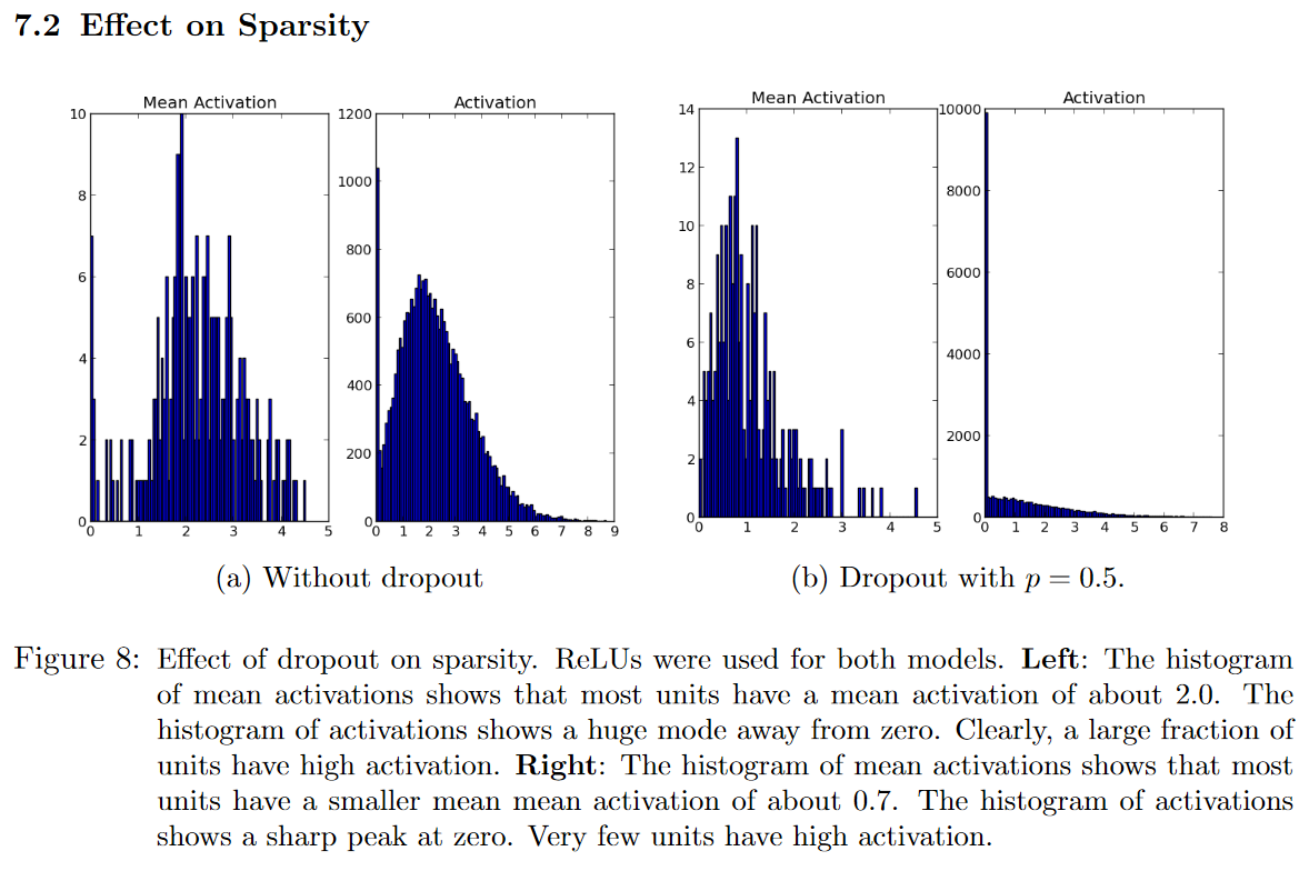
We found that as a side-effect of doing dropout, the activations of the hidden unitsbecome sparse, even when no sparsity inducing regularizers are present. Thus, dropout au-tomatically leads to sparse representations. In a good sparse model, there should only be a few highly activated unitsfor any data case.

Comparing the histograms of activations we can see that fewer hidden units have high activations in Figure 8b compared to Figure 8a, as seen by the significant mass away from zero for the net that does not use dropout. (8-b activation shows about 10k activation compared to 1.2k in 8-a.)

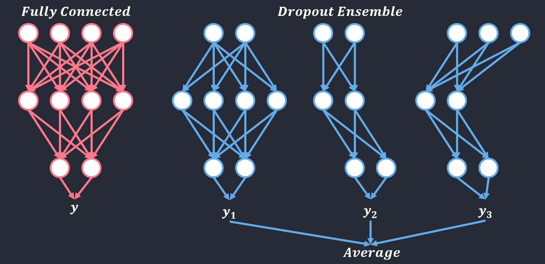
Ensemble Effects

Dropout is training a large ensemble of models (that share parameters).

Ensemble Method

서로 다른 여러 개의 모델을 결합하여 일반화 오류를 줄임

Bagging (Bootstrap Aggregating)

훈련집합을 여러 번 추출하여 서로 다른 훈련집합 구성

Boosting

\(i\)번째 예측기가 틀린 샘플을 \(i+1\)번째 예측기가 잘 인식하도록 연계성 고려

Hyper Parameter Tuning

두 종류의 parameter가 있음

• 내부 매개변수 혹은 가중치
  • 신경망의 경우 가중치
• hyper parameter
  • filter size, stepsize, LR 등

탐색 방식

• Grid Search
• Random Search
• Log space

차원의 저주 문제

• random search가 더 유리.

2차 미분을 이용한 방법

뉴턴 방법

• 2차 미분 정보를 활용
• 1차 미분의 최적화
  • 경사도 사용하여 선형 근사 사용
  • 근사치 최소화
• 2차 미분의 최적화
  • 경사도와 헤시안을 사용하여 2차 근사 사용
  • 근사치의 최소값
• 2차 미분의 단점
  • 변곡점(f’‘=0) 근처에서 매우 불안정한 이동 특성을 보인다는 점
    • 변곡점 근처에서는 f’’ = 0에 가까운 값을 갖기 때문에 스텝(step)의 크기가 너무 커져서 아에 엉뚱한 곳으로 발산해 버릴 수도 있음
  • 이동할 방향을 결정할 때 극대, 극소를 구분하지 않는다는 점
    • 극대점을 향해 수렴할 수도 있음
• 테일러 급수
  • 주어진 함수를 정의역에서 특정 점의 미분계수들을 계수로 가지는 다항식의 극한(멱급수)으로 표현.
• 기계학습이 사용하는 목적함수는 2차 함수보다 복잡한 함수이므로 한 번에 최적해에 도달 불가능
  • 헤시안 행렬을 구해야 함
    • 연산량이 과다하게 필요함
    • 켤레 경사도 방법이 대안으로 제시됨

켤레 경사도 방법 (conjugate gradient method)

직전 정보를 사용하여 해에 빨리 접근

유사 뉴턴 방법

• 경사하강법: 수렴 효율성 낮음
• 뉴턴 방법: 헤시안 행렬 연산 부담
  • 헤시안 H의 역행렬을 근사하는 행렬 M을 사용
• 점진적으로 헤시안을 근사화하는 LFGS가 많이 사용됨.
• 기계학습에서는 M을 저장하는 메모리를 적게 쓰는 L-BFGS를 주로 사용
  • 전체 배치를 통한 갱신을 할 수 있다면, L-BFGS 사용을 고려함

Appendix

Reference

CNN cs231n lecture_8 Optimization: http://cs231n.stanford.edu/slides/2021/lecture_8.pdf
CNN cs231n lecture_3 Loss Functions and Optimization(SGD): http://cs231n.stanford.edu/slides/2021/lecture_3.pdf
CNN cs231n lecture_7 Activation Functions-Data Preprocessing-Weight Initialization-Batch Normalization-Transfer learning: http://cs231n.stanford.edu/slides/2021/lecture_7.pdf
weight initalization: https://silver-g-0114.tistory.com/79
SGD momentumL https://youtu.be/_JB0AO7QxSA
ML: https://wordbe.tistory.com/entry/MLDL-%EC%84%B1%EB%8A%A5-%ED%96%A5%EC%83%81%EC%9D%84-%EC%9C%84%ED%95%9C-%EC%9A%94%EB%A0%B9
Dropout: https://blog.naver.com/PostView.nhn?blogId=laonple&logNo=220818841217&parentCategoryNo=&categoryNo=16&viewDate=&isShowPopularPosts=true&from=search
Dropout paper: https://jmlr.org/papers/volume15/srivastava14a.old/srivastava14a.pdf
2차미분 최적화: https://darkpgmr.tistory.com/149