Chapter3 - Counting 101 - Recursion and Recurrence(1)

Book - Python Algorithms by Magnus Lie Hetland

Chapter 3 - Counting 101

Simple example of how to recursively sum a sequence:

def S(seq, i=0):
    if i == len(seq): return 0
    return S(seq, i+1) + seq[i]

Undertanding how this function works and figuring out its running time are closely related tasks.
The parameter i indicates where the sum is to start. If it’s beyond the end of the sequence, the function returns 0.
Otherwise, it adds the value at position i to the sum of the remaining sequence.
We have a constant amount of work in each execution of s, excluding the recursive call, and it’s executed once for each item in the sequence, so it’s pretty obvious that the running time is linear.

def T(seq, i=0):
    if i == len(seq): return 1
    return T(seq, i+1) + 1

This T function has virtually the same structure as s.
Instead of returning a solution to a subproblem, like s does, it returns the cost of finding that solution.
In this case, I’ve just counted the number of times the if statement is executed. In a more mathematical setting, you would count any relevant operations and use \(\theta(1)\) instead of 1.

>>> seq = range(1,101) 
>>> s(seq) 
5050
>>> T(seq) 
101

>>> for n in range(100): 
...     seq = range(n) 
...     assert T(seq) == n+1

There are no errors, so the hypothesis does seem sort of plausible.

Doing It By Hand

To describe the running time of recursive algorithms mathematically, we use recursive equations, called recurrence relations (점화식).
If our recursive algorithm is like S in the previous section, then the recurrence relation is defined somewhat like T.
we implicitly assume that T(k) = Θ(1), for some constant k. That means we can ignore the base cases when setting up our equation (unless they don’t take a constant amount of time), and for S, our T can be defined as follows: \[ T(n) = T(n-1) + 1 \]
This means that the time it takes to compute S(seq, i), which is T(n), is equal to the time required for the recursive call S(seq, i+1), which is T (n–1), plus the time required for the access seq[i], which is constant, or Θ(1).

\(\theta(n) = \theta(n-1) + \theta(1)\).
By removing constant \(\theta(1)\),
we can get \(\theta(n) = \theta(n-1)\)

As we know that \(T(n) = T(n-1)+1\), replace n with n-1, then:

\[\begin{align} T(n) & = T(n-1) + 1 \\ & = T(n-2) + 1 + 1 \\ & = T(n-3) + 1 + 1 + 1 \\ \end{align}\]

The fact that \(T(n–2) = T (n–3) + 1\) (the two boxed expressions) again follows from the original recurrence relation. It’s at this point we should see a pattern: Each time we reduce the parameter by one, the sum of the work (or time) we’ve unraveled (outside the recursive call) goes up by one.

If we unravel T (n) recursively i steps, we get the following:
\[ T(n) = T(n-i) + i\]
where the level of recursion is expressed as a variable.

What we do is go right up to the base case and try to make \(T(n–i)\) into \(T(1)\), because we know, or implicitly assume, that \(T(1)\) is \(\theta(1)\), which would mean we had solved the entire thing. And we can easily do that by setting i = n–1:

\[\begin{align} T(n) & = T(n-(n-1)) + (n-1)\\ & = T(1) + n - 1\\ & = \theta(1) + n - 1\\ & = \theta(n)\\ \end{align}\]

Found that s has a linear running time.

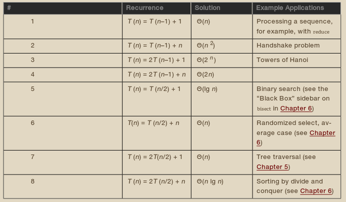
Some Recurrences [Table 3-1]

[Table 3-1]

⛔ Caution ⛔

This method, called the method of repeated substitutions (or sometimes the iteration method ), is perfectly valid, if you’re careful. However, it’s quite easy to make an unwarranted assumption or two, especially in more complex recurrences. This means you should probably treat the result as a hypothesis and then check your answer using the techniques described in the section “Guessing and Checking” later in this chapter.

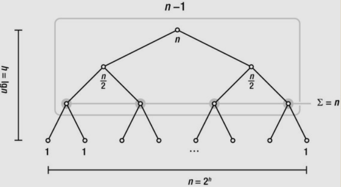
Recurrence 5 [Table 3-1]

a perfect binary tree

\[\begin{align} T(n) & = T(n/2) + 1 \\ & = {T(n/4) + 1} + 1 \\ & = {T(n/8) + 1} + 1 + 1 \\ \end{align}\]

Test

Unraveling Recurrence

This stepwise unraveling (or repeated substitution) is just the first step of our solution method. The general approach is as follows:

1. Unravel the recurrence until you see a pattern.
2. Express the pattern (usually involving a sum), using a line number variable, i.
3. Choose i so the recursion reaches its base case (and solve the sum).

The first step is what we have done already. Let’s have a go at step 2:
\[ T(n) = T(n/2^{i}) + \sum_{k=1}^{i}1 \]
For each unraveling (each line further down), we halve the problem size (that is, double the divisor) and add another unit of work (another 1).
We know we have i ones, so the sum is clearly just i. I’ve written it as a sum to show the general pattern of the method here. \(\sum_{k=1}^{i}1 = i\).

To get to the base case of the recursion, we must get \(T (n/2^{i} )\) to become, say, \(T(1)\). That just means we have to halve our way from n to 1, which should be familiar by now: The recursion height is logarithmic, or \(i = \log n\).
Insert that into the pattern, and you get that \(T(n)\) is, indeed, \(\theta(\log n)\).

Recurrence 6 [Table 3-1]

\(\begin{align} T(n) & = 2T(n/2) + n \\ & = 2{2T(n/4) + n/2} + n \\ & = 2(2\{2T(n/8) + n/4\} + n/2) + n \\ ... \\ & = 2^{i}T(n/2^{i}) + n\cdot i \\ \end{align}\)

Set \(i = logn\). Assuming that \(T(1) = 1\), we get the following:
\[ T(n) = 1 + \sum_{k=0}^{\log n-1}(n/2^{k}) = \sum_{k=0}^{\log n}(n/2^{k}) \]

Assert (가정 설정문)

assert는 뒤의 조건이 True가 아니면 AssertError를 발생한다.

Assert 사용하는 이유:

어떤 함수는 성능을 높이기 위해 반드시 정수만을 입력받아 처리하도록 만들 수 있다. 이런 함수를 만들기 위해서는 반드시 함수에 정수만 들어오는지 확인할 필요가 있다. 이를 위해 if문을 사용할 수도 있고 ‘예외 처리’를 사용할 수도 있지만 ‘가정 설정문’을 사용하는 방법도 있다.

아래 코드는 함수 인자가 정수인지 확인하는 코드이다.

lists = [1, 3, 6, 3, 8, 7, 13, 23, 13, 2, 3.14, 2, 3, 7]

def test(t):
    assert type(t) is int, '정수 아닌 값이 있네'

for i in lists:
    test(i)
#결과
AssertionError: 정수 아닌 값이 있네

Assert format

assert 조건, ‘메시지’
‘메시지’는 생략할 수 있다.
assert는 개발자가 프로그램을 만드는 과정에 관여한다. 원하는 조건의 변수 값을 보증받을 때까지 assert로 테스트 할 수 있다.
이는 단순히 에러를 찾는것이 아니라 값을 보증하기 위해 사용된다.
예를 들어 함수의 입력 값이 어떤 조건의 참임을 보증하기 위해 사용할 수 있고 함수의 반환 값이 어떤 조건에 만족하도록 만들 수 있다. 혹은 변수 값이 변하는 과정에서 특정 부분은 반드시 어떤 영역에 속하는 것을 보증하기 위해 가정 설정문을 통해 확인 할 수도 있다.
이처럼 실수를 가정해 값을 보증하는 방식으로 코딩 하기 때문에 이를 ‘방어적 프로그래밍’이라 부른다.

>>> assert 2 + 2 == 4
>>> assert 2 + 2 == 3
Traceback (most recent call last):
  File "<interactive input>", line 1, in <module>
AssertionError

>>> assert 1 == False, "That can't be right."
Traceback (most recent call last):
  File "<interactive input>", line 1, in <module>
AssertionError: That can't be right.

Recurrence Relation (점화식)

In mathematics, a recurrence relation is an equation that recursively defines a sequence or multidimensional array of values, once one or more initial terms are given; each further term of the sequence or array is defined as a function of the preceding terms.

python assert: https://wikidocs.net/21050
docs: https://python-reference.readthedocs.io/en/latest/docs/statements/assert.html
recurrence relation: https://en.wikipedia.org/wiki/Recurrence_relation