Build Basic Generative Adversarial Networks (GANs)

Generative Adversarial Networks (GANs) Specialization offered by DeepLearning.AI

Generative Models

• Variational Autoencoder(VAE)
• Generative Adversarial Network(GAN)

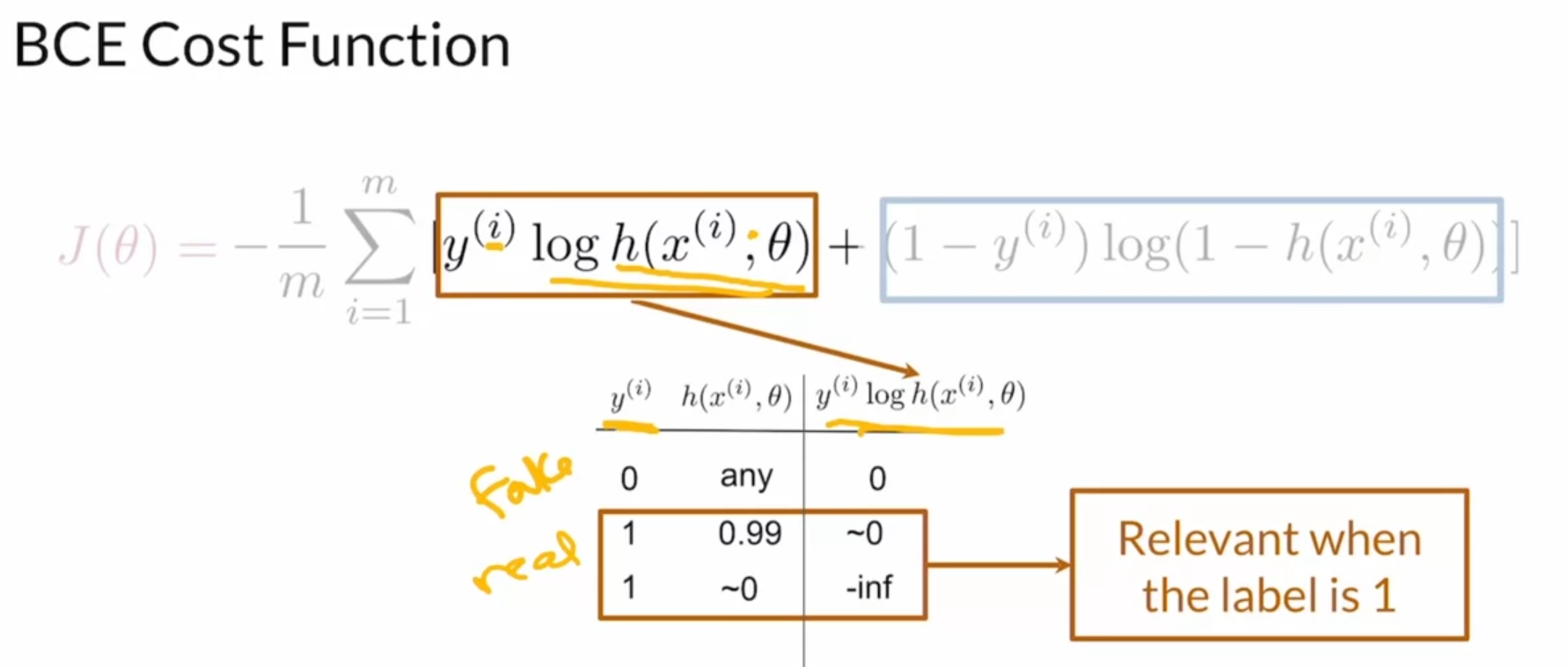
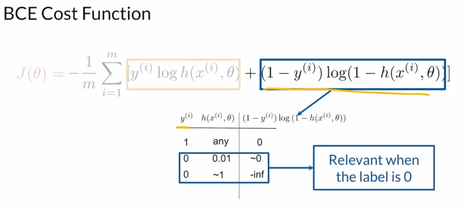
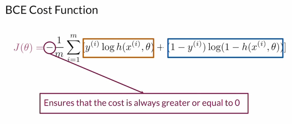
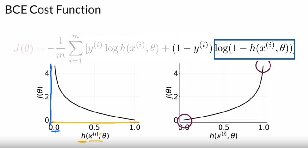
BCE Cost Function

GAN Overall

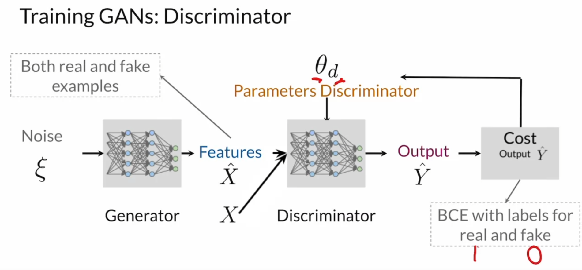
Discriminator

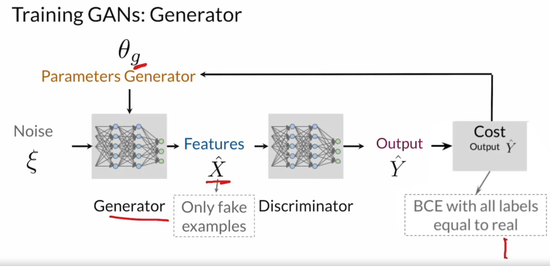
Generator

Improve Together

It’s important to keep in mind that both models should improve together and should be kept at similar skill levels from the beginning of training.

And the reasoning behind this is largely because of the discriminator. The discriminator has a much easier task, it’s just trying to figure out which ones are real, which ones are fake, as opposed to model the entire space of what a class could look like.

If discriminator is superior (all Fake)

If you had a discriminator that is superior than the generator, like super, super good, you’ll get predictions from it telling you that all the fake examples are 100% fake.
Well, that’s not useful for the generator, the generator doesn’t know how to improve. Everything just looks super fake, there isn’t anything telling it to know which direction to go in.

If generator is superior (all Real)

Meanwhile, if you had a superior generator that completely outskills the discriminator, you’ll get predictions telling you that all the generated images are 100% real.

Creating Own GAN

• torch.randn vs torch.rand
  • torch.randn: Returns a tensor filled with random numbers from a normal distribution with mean 0 and variance 1
  • torch.rand: Returns a tensor filled with random numbers from a uniform distribution on the interval [0, 1)[0,1)

Activations

differentiable and non-linear function

1. Differentiable for backpropagation (provide gradient)
2. Non-linear to compute complex features, if not simple linear regression.

Common Activation Functions

• ReLU: \(g^{[l]}(z^{[l]}) = max(0, z^{[l]})\), \([l]\): l-th layer
  • Dying ReLU problem: end of learning
• LeakyReLU: \(g^{[l]}(z^{[l]}) = max(az^{[l]}, z^{[l]})\)
  • the slope(\(a\)) is treated as a hyperparameter typically set to 0.1, meaning the leak is quite small relative to the positive slope still.
  • this slope solves the dying ReLU problem.
• Sigmoid: \(g^{[l]}(z^{[l]}) = \frac{1}{1+e^{-z^{[l]}}}\)
  • values between 0 and 1
  • vanishing gradient problems: the sigmoid activation function isn’t used very often in hidden layers because the derivative of the function approaches zero at the tails of this function.
• Tanh: \(g^{[l]}(z^{[l]}) = \tanh(z^{[l]})\)
  • values between -1 and 1
  • same issue as Sigmoid
• In short, ReLU with the dying ReLU problem, and sigmoid and tanh with the vanishing ingredient in saturation problems.

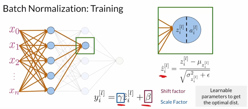
Batch Normalization (Covariate Shift)

• The result of having different distributions impacts away your neural network learns. For example, if it’s trying to get to this local minimum here and it has these very different distributions across inputs, this cost function will be elongated. So that changes to the weights relating to each of the inputs will have kind of a different effect of varying impact on this cost function. And this makes training fairly difficult, makes it slower and highly dependent on how your weights are initialized.
• Additionally, if new training or test data has, so the state is distribution kind of shifts or changes in some way, then the form of the cost function could change too.
• Even if the ground truth of what determines whether something’s a cat or not stays exactly the same. That is the labels on your images of whether something is a cat or not has not changed. And this is known as covariate shift.
• Normalized, meaning, the distribution of the new input variables x1 prime and x2 prime will be much more similar with say means equal to 0 and a standard deviation equal to 1. Then the cost function will also look smoother and more balanced across these two dimensions.
• And as a result training would actually be much easier and potentially much faster.
• Additionally, no matter how much the distribution of the raw input variables change, for example from training to test, the mean and standard deviation of the normalized variables will be normalized to the same place. So around a mean of 0 and a standard deviation of 1.
• And using normalization, the effect of this covariate shift will be reduced significantly. And so those are the principle effects of normalization of input variables, smoothing that cost function out in reducing the covariate shift.

Covariate Shift

Covariate shift means that the distributions of some variables are dependent on another.

Internal Covariate Shift

• Neural networks are actually susceptible to something called internal covariate shift, which just means it’s covariate shift in the internal hidden layers.
• Batch normalization seeks to remedy the situation. And normalizes all these internal nodes based on statistics calculated for each input batch. And this is in order to reduce the internal covariate shift. And this has the added benefit of smoothing that cost function out and making the neural network easier to train and speeding up that whole training process.

Batch Normalization Procedure

Appendix

Reference