ML basics - Probability Part 2

Deep Learning Model’s Outcome is the Probability of the Variable X

Rules of Probability

Product Rule

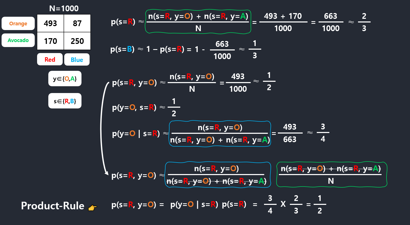\[ p(s,y) = p(y|s)p(s) \] \[ p(y,s) = p(s|y)p(y) \]

Eventhough we don’t know the intersection probability of R and O,
if there are p(y=O|s=R) and p(s=R), we can get the prob of p(s=R, y=O)

Sum Rule

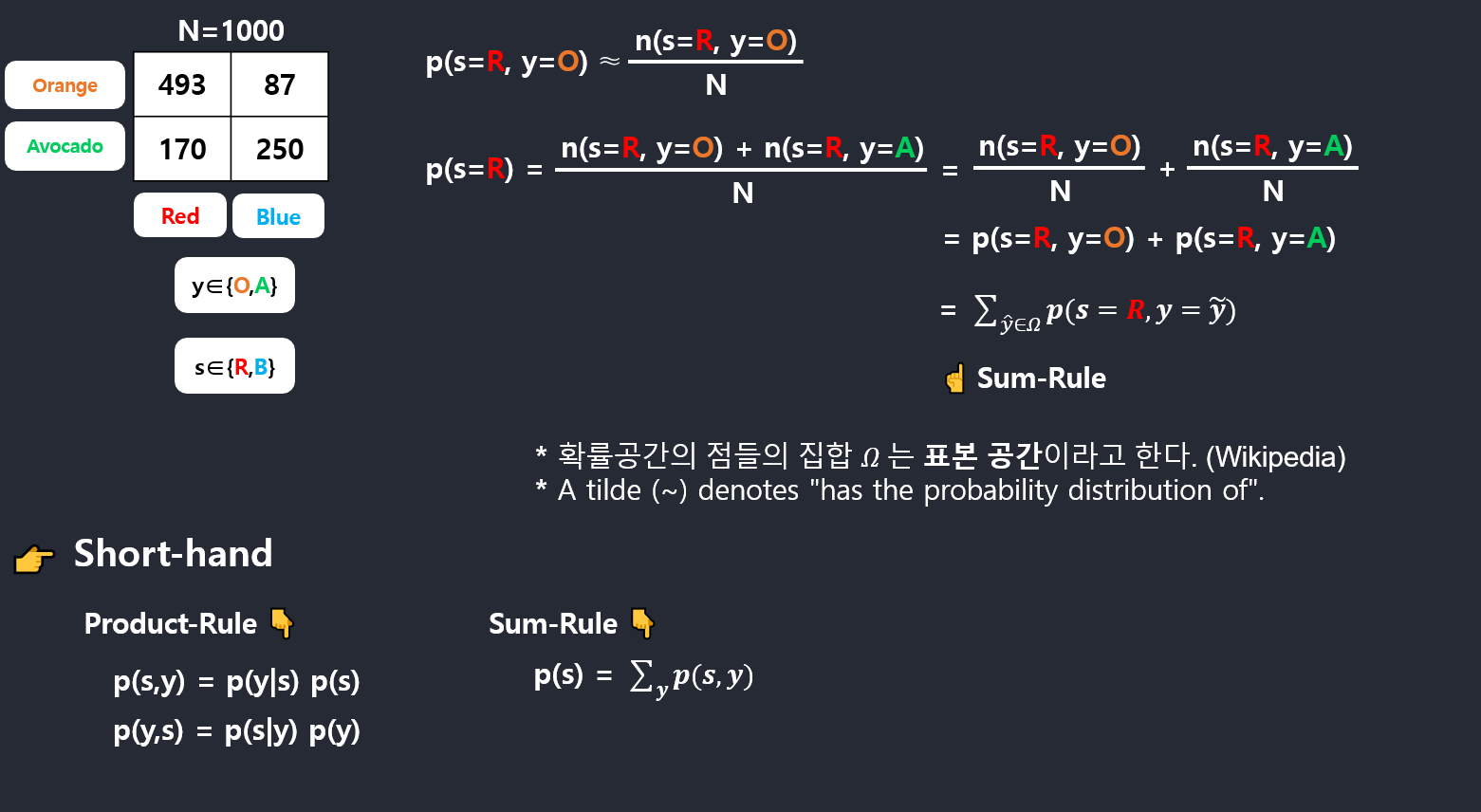
\[ p(X) = \sum_{Y}\ p(X,Y) \]

Bayes Theorem

• posterior
• likelihood
• prior
• normalization
• marginal prob dist
• Conditional prob dist

Why Bayes Theorem is useful?

It’s all about dependency.
What I learned about intersection in school is that \(P(A \cap B) = P(A)\ P(B)\).
This is only true when those two event A and B are independent.
However, in reality this is not pleasible, this is why bayes theorm comes.

\[ P(H\mid E) = \frac{P(H)P(E\mid H)}{P(E)} \]

3B1B example (Librarian or Farmer)

Prior state:
The ratio is 20:1 (farmer:librarian).

Is Steve more likely to be a librarian or a farmer?
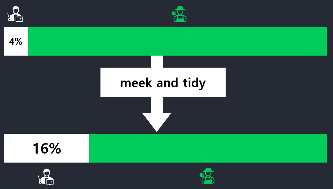
“Steve is very shy and withdrawn, invariably helpful but with very little interest in people or in the world of reality. A meek and tidy soul, he has a need for order and structure, and a passion for detail.”
Before given the information about meek and tidy, people decribe steve as more likely a farmer.
However, after that, people view as a librarian.
Accoding to Kahneman and Tversky, this is irrational.
What’s important is that almost no one thinks to incorporate information about the ratio of farmers to librarians into their judgements.

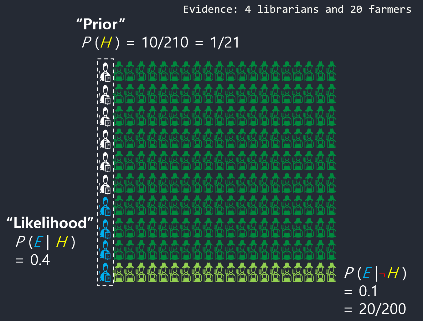
• Sample 10 librarians and 200 farmers.
• Hear meek and tidy description.
• Your instinct: 40% of librarians and 10% of farmers
• Estimate: 4 librarians and 20 farmers

The prob of random person who fits this description is a librarian is 4/24, or 16.7%.
\[ P(Librarian\ given\ Description) = \frac{4}{4+20} \thickapprox 16.7%\]

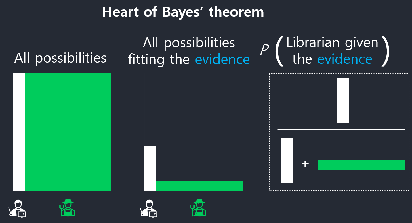
Even if you think a librarian is 4 times as likely as a farmer to fit this description(40% Vs. 10%), that’s not enough to overcome the fact that there are way more farmers (prior state ratio).
The key underlying Bayes’ theorem is that new evidence does not completely determine your beliefs. It should update prior beliefs.

Heart of Bayes’ Theorem

When to use Bayes’ Theorem

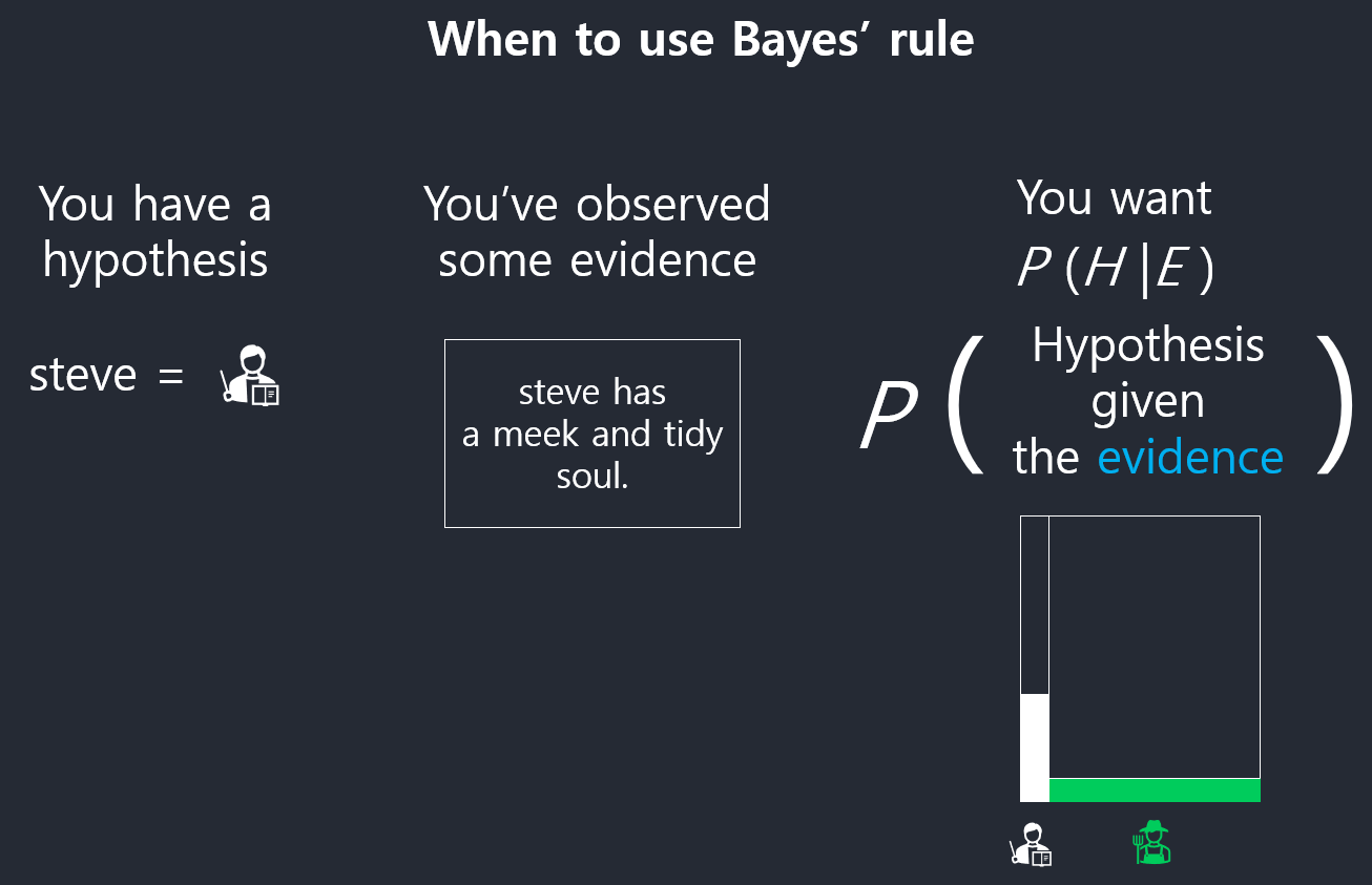
Prior and likelihood

Posterior

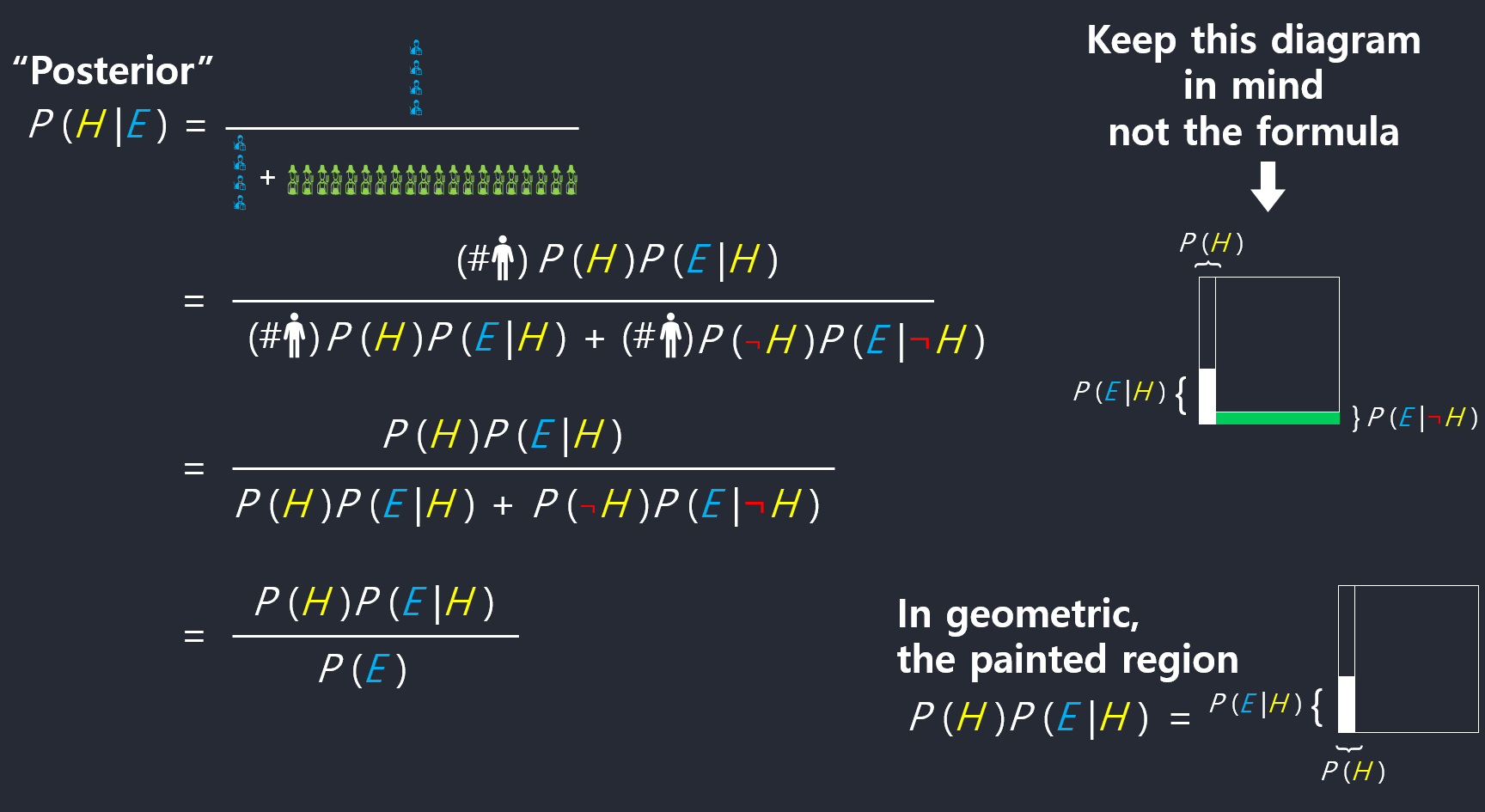
Normalization

In probability theory, a normalizing constant is a constant by which an everywhere non-negative function must be multiplied so the area under its graph is 1, e.g., to make it a probability density function or a probability mass function.
베이즈 정리에서 \(P(\mathbb E)\) 가 normalizing constant 라고 보면된다.

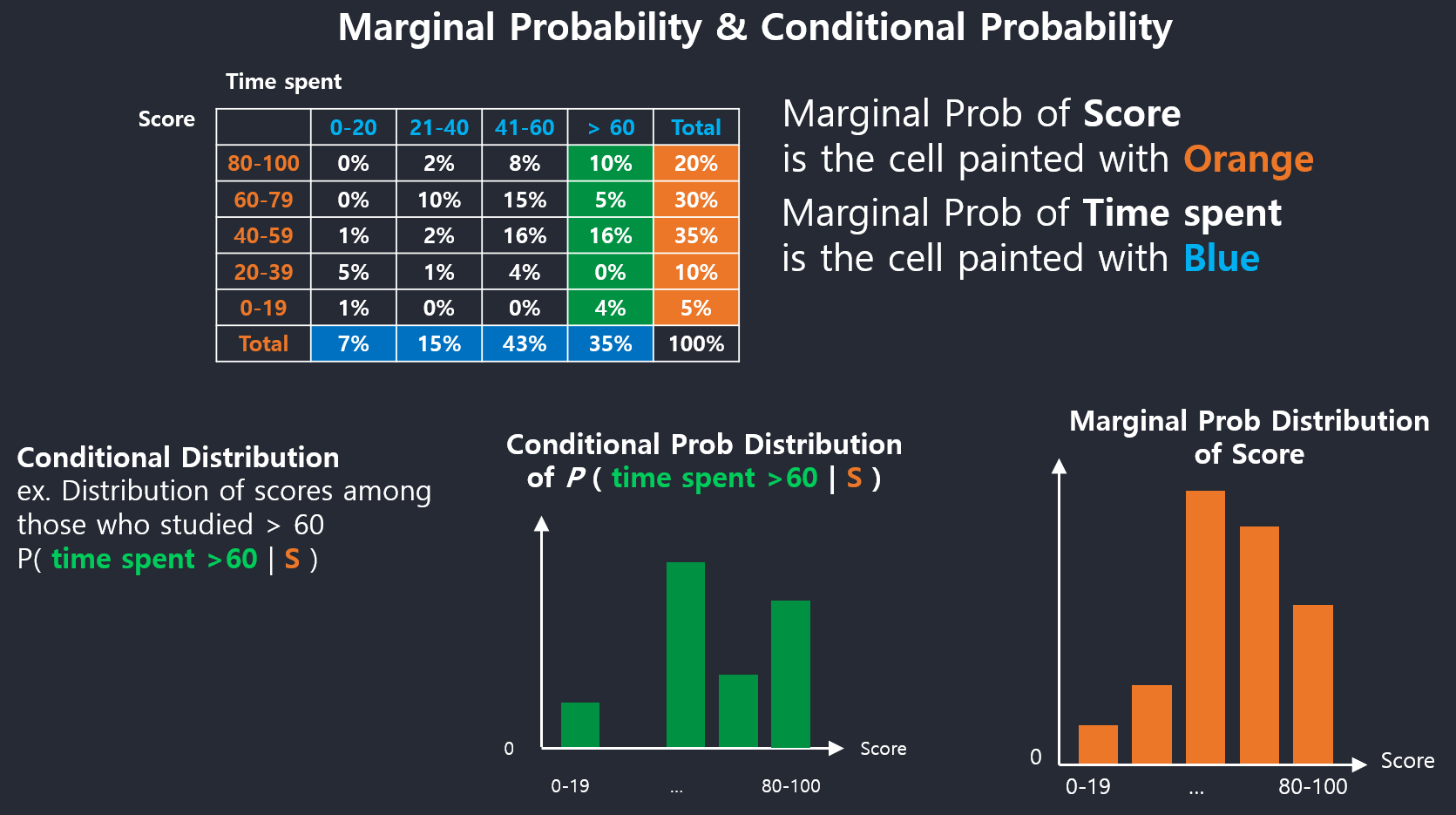
Marginal Probaility Distribution & Conditional Probaility Distribution

Marginal stands for the marginal of the table.
Marginal probability doesn’t tell about the specific probability(i.e. each cell.)

Functions of Random Variables

Joint PDF

k차원의 확률변수 벡터 \(\mathbf x = (x_{1} , … , x_{k})\) 가 주어졌을때,
확률변수벡터 \(\mathbf y = (y_{1} , … , y_{k})\) 를 정의한다.
\(\mathbf y =\mathbf g(\mathbf x)\) 로 나타낼 수 있다.
ex. \(\mathbf y_{1} =\mathbf g_{1}(x_{1} , … , x_{k})\)
만약 \(\mathbf y =\mathbf g(\mathbf x)\) 가 일대일 변환인 경우,
\(\mathbf y\)의 Joint PDF는
\[ P_{\mathbf y}\ (y_{1} , … , y_{k}) = P_{\mathbf x}\ (x_{1} , … , x_{k})\ |J| \]
\(J\) is the matrix of all its first-order partial derivatives.(wikipedia)

Jacobian Matrix

Jacobian Matrix: is the matrix of all first-order partial derivatives of a multiple variables vector-valued function. When the matrix is a square matrix, both the matrix and its determinantare referred to as the Jacobian in literature. The Jacobian is then the generalization of the gradient for vector-valued functions of several variables.

first-order partial derivatives: The first order derivative of a function represents the rate of change of one variable with respect to another variable. For example, in Physics we define the velocity of a body as the rate of change of the location of the body with respect to time. Here location is the dependent variable on the other hand time is the independent variable. To find the velocity, we need to compute the first order derivative of the location. Similarly, we can this concept for computing rate of dependency of one variable over the other. https://www.toppr.com/guides/fundamentals-of-business-mathematics-and-statistics/calculus/derivative-first-order/

Note that when m=1 the Jacobian is same as the gradient because it is a generalization of the gradient. https://math.stackexchange.com/questions/1519367/difference-between-gradient-and-jacobian

아무리 복잡한 함수라도 Jacobian Matrix를 구할 수 있다면, 새로 주어진 확률 변수에 대해서 밀도함수를 구할 수 있다는 것이 강력한 힘이다.

비선형변환이지만 작은 영역에서는 선형변환이지 않을까.
국소적 영역에서 선형변환으로 approx할 수 있지 않을까.

Inverse CDF Technique

In probability and statistics, the quantile function, associated with a probability distribution of a random variable, specifies the value of the random variable such that the probability of the variable being less than or equal to that value equals the given probability. It is also called the percent-point function or inverse cumulative distribution function.

By cumulative distribution function we denote the function that returns probabilities of \(X\) being smaller than or equal to some value \(x\),
\[ Pr(X \le x) = F(X) \]
This function takes as input \(x\) and returns values from the \([0,1]\) interval (probabilities)—let’s denote them as \(p\). The inverse of the cumulative distribution function (or quantile function) tells you what \(x\) would make \(F(x)\) return some value \(p\), \[ F^{−1}(p) = x \]

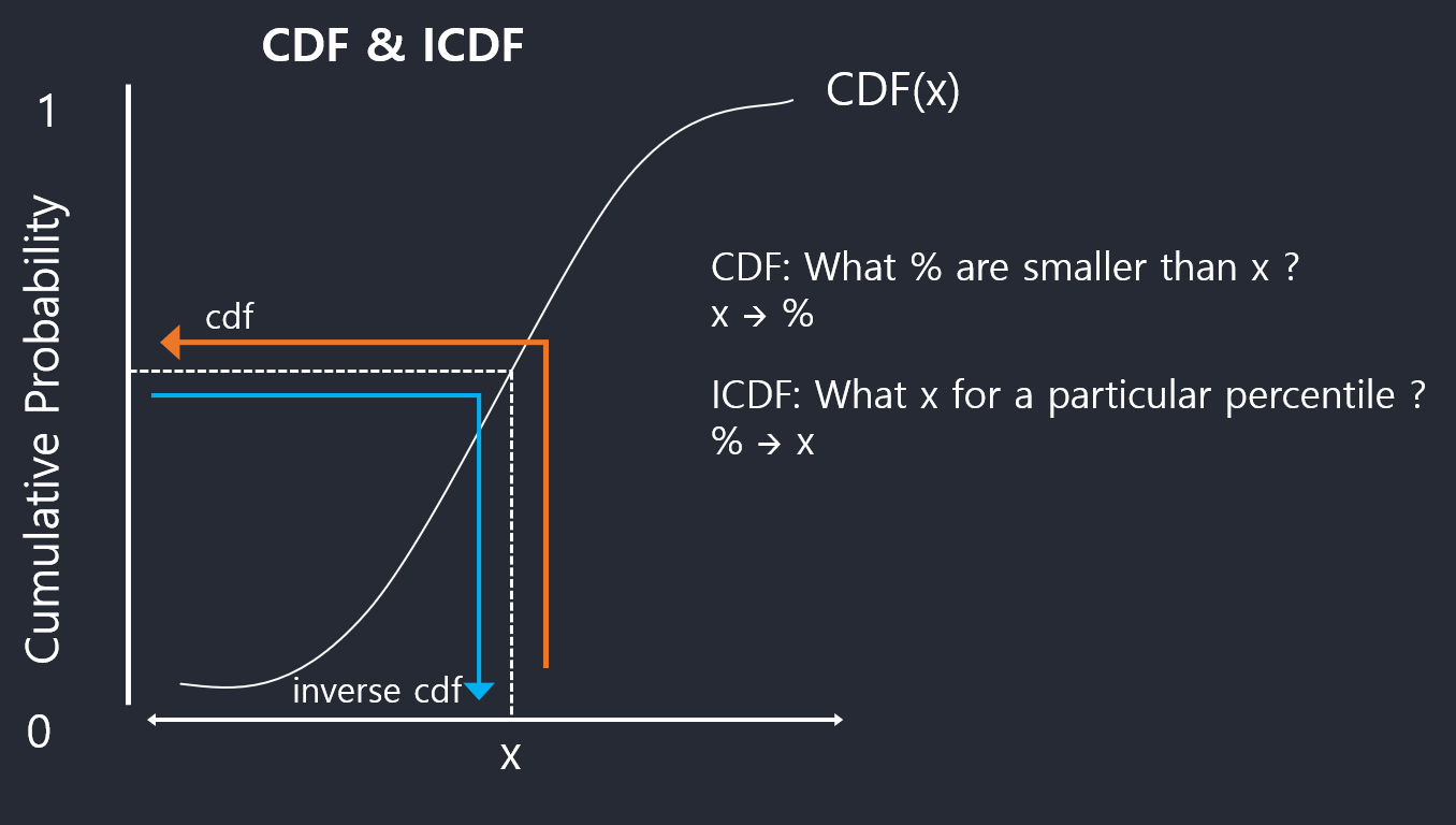
In short:
CDF: x -> prob
ICDF: prob -> x

Expectations

Discrete Distribution

Expectation of Discrete Distribution can be interpreted as weighted sum of\(p(x_{i})\).
\[ \mathbb E[X] = \sum_{x_{i}\in \omega}x_{i}\ p(x_{i}) \]
or
\[ \mathbb E[f] = \sum_{x}p(x)\ f(x) \]

Continuous Distribution

\[ \mathbb E[X] = \int\ x\ f(x)\ dx \]
or
\[ \mathbb E[f] = \int\ p(x)\ f(x)\ dx \]

Multiple Random Variables

두 개의 변수 x, y의 경우:
\[ \mathbb E_{x}{[}f(x,y){]} = \sum_{x}f(x,y)p(x) \]
여기서 x에 관해서 합을 해버리거나 적분을 해버리기 때문에 결과는 y에 관한 것들만 남게 된다.
따라서 y에 대한 함수이다.

두 개의 변수 모두에 대해 기대값을 구할때는 joint pdf가 주어지기 때문에 더하면 된다. \[ \mathbb E_{x,y}{[}f(x,y){]} = \sum_{y}\sum_{x}f(x,y)p(x,y)\]

Conditional Expectation

\[ \mathbb E_{x}{[}f|y{]} = \sum_{x}f(x)p(x|y) \]

Variance

Variance is the expectation of the squared deviation of a random variable from its mean. The variance is the square of the standard deviation.
\[ var[f] = \mathbb E{[}(f(x)-\mathbb E{[}f(x){]})^{2}{]} = \mathbb E{[}f(x)^{2}{]} - \mathbb E{[}f(x){]} ^{2} \]
\[ var[x] = \mathbb E{[}x^{2}{]} - \mathbb E{[}x{]} ^{2} \]

Covariance

Covariance is a measure of the joint variability of two random variables. The sign of the covariance shows the tendency in the linear relationship between the variables.

for random variable x and y:

\[\begin{align} cov {[}x,y{]} &= \mathbb E_{x,y}{[}{x-\mathbb E{[}x{]} }{y-\mathbb E{[}y{]} }{]} \\ &= \mathbb E_{x,y}{[}xy{]} - \mathbb E{[}x{]} \mathbb E{[}y{]} \\ \end{align}\]

for vector of random variable \(\mathbf x\) and \(\mathbf y\):

\[\begin{align} cov {[}\mathbf x,\mathbf y{]} &= \mathbb E_{\mathbf x,\mathbf y}{[}{\mathbf x-\mathbb E{[}\mathbf x{]} }{y^{T} -\mathbb E{[}\mathbf y^{T}{]} }{]} \\ &= \mathbb E_{\mathbf x,\mathbf y}{[}\mathbf x\mathbf y^{T}{]} - \mathbb E{[}\mathbf x{]} \mathbb E{[}\mathbf y^{T}{]} \\ cov {[}\mathbf x,\mathbf y{]} &= cov {[}\mathbf x,\mathbf x{]} \end{align}\]

Gaussian Distribution

정규 분포 또는 가우스 분포(Gaussian distribution)는 연속 확률 분포의 하나이다. 정규분포는 수집된 자료의 분포를 근사하는 데에 자주 사용되며, 이것은 중심극한정리에 의하여 독립적인 확률변수들의 평균은 정규분포에 가까워지는 성질이 있기 때문이다.
정규분포는 2개의 매개 변수 평균 \(\mu\) 과 표준편차 \(\sigma\) 에 대해 모양이 결정되고, 이때의 분포를 \(N(\mu ,\sigma ^{2})\)로 표기한다. 특히, 평균이 0이고 표준편차가 1인 정규분포 \(N(0,1)\)을 표준 정규 분포(standard normal distribution)라고 한다.

가우시안 분포의 확률밀도함수(PDF):
\[ \mathcal{N}(x|/mu, \sigma ^{2}) = \frac{1}{(2\pi\sigma^{2})^{1/2}} exp \left(-\frac{(x-\mu)^{2}}{2\sigma^{2}}\right) \]

확률밀도함수가 주어졌을 때, 그 함수를 \(-\infty\)부터 \(\infty\)까지 적분했을때 그 값이 1이 되면 이 밀도함수는 normalized.
\[ \int_{-\infty}^{\infty}\ \mathcal{N}(x|\mu, \sigma^{2})dx = 1 \]

Expectation

\[ \mathbb E{[}x{]} = \mu \]

Variance

\[ var{[}x{]} = \sigma^{2} \]

Maximum Likelihood Solution

\(\mathbf X = (x_{1},...,x_{N})^{T}\)가 독립적으로 같은 가우시안분포로부터 추출된 N개의 샘플들이라고 할 떄,

\[\begin{align} p(\mathbf X|\mu,\sigma^{2}) & = p(x_{1},...,x_{N}|\mu, \sigma^{2}) \\\\ & = \Pi_{n=1}^{N}\ \mathcal{N}(x|\mu, \sigma^{2}) \\\\ & = N(x_{1}|\mu, \sigma^{2})\times\ N(x_{1}|\mu, \sigma^{2})\times\ ...\ \times\ N(x_{N}|\mu, \sigma^{2}) \end{align}\]

$$p(\mathbf X

\mu,\sigma^{2})\(이 값을 최대화 시키는\)\mu\(와\)\sigma$$를 찾으려고 한다.

\(\mu\)의 Maximum Likelihood Solution

자연로그 \(\ln\)를 씌워서 푼다:
\[ \ln\ p(\mathbf X|\mu,\sigma^{2}) = -\frac{1}{2\sigma^{2}} \sum_{n=1}^{N}(x_{n}-\mu)^{2} -\ \frac{N}{2}\ln\sigma^{2} -\ \frac{N}{2}\ln(2\pi) \]

최대우도해를 구하기 위해서 로그를 씌운 후 \(\mu\)값으로 미분한다.
\(\begin{align} \frac{\partial}{\partial\mu}\ln\ p(\mathbf X|\mu,\sigma^{2}) &= \frac{\partial}{\partial\mu} \left\{-\frac{1}{2\sigma^{2}} \sum_{n=1}^{N}(x_{n}-\mu)^{2} - \frac{N}{2}\ln\ \sigma^{2} - \frac{N}{2}\ln(2\pi) \right\} \\\\ &= -\frac{1}{2\sigma^{2}} \sum_{n=1}^{N}2(x_{n}-\mu)\cdot(-1) \\\\ &= \frac{1}{\sigma^{2}}\left\{ \left(\sum_{n=1}^{N}x_{n}\right) - N\mu \right\} \end{align}\)

\[ \mu_{ML} = \frac{1}{N} \sum_{n=1}{N}x_{n} \]
*ML: Maximum Likelihood
가우시안 분포의 평균값을 데이터로부터 찾고 싶은데 N값을 관찰했을때 N개의 값을 평균을 내면 이 함수의 평균이 되지 않을까.

\(\sigma^{2}\)의 Maximum Likelihood Solution

\(y=\sigma^{2}\)
최대우도해를 구하기 위해서 로그를 씌운 후 \(\sigma^{2}\)값으로 미분한다.

\[\begin{align} \frac{\partial}{\partial y}\ln\ p(\mathbf X|y,\sigma^{2}) &= \frac{\partial}{\partial y} \left\{-\frac{1}{2}y^{-1} \sum_{n=1}^{N}(x_{n}-\mu_{ML})^{2} - \frac{N}{2}\ln y\ \sigma^{2} - \frac{N}{2}\ln(2\pi) \right\} \\\\ &= \frac{1}{2}y^{-2} \sum_{n=1}^{N}2(x_{n}-\mu_{ML})^{2} - \frac{N}{2}y^{-1} \\\\ \end{align}\]

\[ y_{ML} = \sigma_{ML}^{2} = \frac{1}{N} \sum_{n=1}{N}(x_{n}-\mu_{ML})^{2} \]

Curve Fitting: Probabilistic Prospect

Train data:
\(\mathbf x = (x_{1} , … , x_{N})^{T}, \mathbf t = (t_{1} , … , t_{N})\)

목표값 \(\mathbf t\)의 불확실성을 다음과 같이 확률분포로 나타낸다.
\[ p(t|x, \mathbf w, \beta) = \mathcal{N}(t|y(x,\mathbf w),\beta^{-1})\]

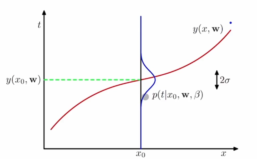
\(x_{0}\)라는 값에 대해서,
\(\mathbf w\)를 파라미터로 하는 \(y\) 함수의 값이 있지만,
그 값에 대한 불확실성을 나타내기 위해 확률을 가정한다.
\(x_{0}\)가 주어졌을 때 \(t\)의 확률은 가우시안 분포를 따른다고 가정한다.(그림에서 파란선)

\(\mathcal{N}(t\mid y(x,\mathbf w),\beta^{-1})\):
\(t\mid y(x,\mathbf w)\)인 근사식을 평균으로 가지고, \(\beta^{-1}\)을 분산으로 가지는 가우시안 분포.
따라서 이것의 확률 분포는 \(p(t\mid x, \mathbf w, \beta)\)이다.

Maximum Likelihood of \(\mathbf w\)

파라미터는 \(\mathbf w, \beta\)이고 파라미터들의 최대우도해를 구해보자.

• Likelihood Function:
  \[ p(\mathbf t|\mathbf X, \mathbf w, \beta) = \Pi_{n=1}^{N}\ \mathcal{N}(t_{n}|y(x_{n}, \mathbf w), \beta^{-1}) \]
• Log Likelihood Function:
  \[ \ln\ p(\mathbf t|\mathbf X,\mathbf w,\beta) = -\frac{\beta}{2} \sum_{n=1}^{N} (y(x_{n}, \mathbf w)-t_{n})^{2} -\ \frac{N}{2}\ln\beta -\ \frac{N}{2}\ln(2\pi) \]

\(\mathbf w\)에 관해서 우도함수를 최대화시키는 것은
제곱합 오차함수(sum-of-squares)(\(\sum_{n=1}^{N} (y(x_{n}, \mathbf w)-t_{n})^{2}\))를 최소화 시키는 것과 동일하다.
\[ \sum_{n=1}^{N} (y(x_{n}, \mathbf w)-t_{n})^{2} \]

Maximum Likelihood of \(\beta\)

\[ \frac{1}{\beta_{ML}} = \frac{1}{N} \sum_{n=1}{N}(y(x_{n},\mathbf w_{ML})-t_{n})^{2} \]

Predictive Distribution

가정:
\[ p(t|x, \mathbf w, \beta) = \mathcal{N}(t|y(x,\mathbf w),\beta^{-1})\]

Maximum Likelihood Solution:
\[ p(t|x, \mathbf w_{ML}, \beta_{ML}) = \mathcal{N}(t|y(x,\mathbf w_{ML}),\beta_{ML}^{-1})\]

Bayesian Curve Fitting

Prior

파라미터 \(\mathbf w\)의 사전확률(prior) 가정:

\[p(\mathbf w\mid \alpha) = \mathcal{N}(\mathbf w\mid 0, \alpha^{-1}I) = \left(\frac{\alpha}{2\pi}\right)^{(M+1)/2}\ exp \left\{ -\frac{\alpha}{2}\mathbf w^{T}\mathbf w \right\}\]

\(\mathbf w\)의 사후확률(posterior)은 우도함수(likelihood)와 사전확률의 곱에 비례한다.
\[ p(\mathbf w\mid \mathbf X,\ \mathbf t,\ \alpha,\ \beta) \propto p(\mathbf t\mid \mathbf X, \mathbf w,\beta)p(\mathbf w\mid \alpha)\]

• \(A \propto B\): A is directly proportional to B

이 사후확률을 최대화시키는 것은 아래 함수를 최소화시키는 것과 동일하다.

\[\frac{\beta}{2}\sum_{n=1}{N}\{ y(x_{n}, \mathbf w)-t_{n} \}^{2} + \frac{\alpha}{2}\mathbf w^{T}\mathbf w\]

이것은 regularization에서 제곱합 오차함수를 최소화 시키는 것과 동일하다.
Regularization:

\(\begin{align}\tilde{E}(w) = \frac{1}{2}(\ \sum_{n=1}^{N} \{y(x_{n},w)-t_{n}\} ^{2} + \lambda\sum_{n=1}^{N}w_{n}^{2}\ )\end{align}\)
이렇게 되는데 여기서 \(\lambda\) 를 통해서 고차항의 parameters를 0에 가까운 값으로 만들어 주어 적당한 2차항의 함수로 만들어주는 정규화를 실행.
\(\lambda\) 값이 커질수록 \(\lVert \mathbf{w} \rVert^{2}\)의 값을 작게 만들어준다. https://marquis08.github.io/devcourse2/probability/mathjax/ML-basics-Probability-1/

통찰:
t에 관해서 가우시안 분포를 가정했을때, 최대우도를 만들어내는 \(\mathbf w\)가 결국 제곱합 오차함수를 푸는 해와 동일.
추가적으로 \(\mathbf w\)에 관해서도 가우시안 분포를 가정했을때, 사후확률을 최대화 시키는 것은 규제화부분을 포함시켜서 \(\mathbf w\) 구하는 것과 동일하다.

Bayesian Curve Fitting

이제까지 \(t\)의 예측 분포를 구하기 위해 여전히 \(\mathbf w\)의 점추정에 의존해 왔다. 완전한 베이지안 방법은 \(\mathbf w\)의 분포로부터 확률의 기본법칙만을 사용해서 \(t\)의 예측분포를 유도한다.
\[ p(t\mid x, \mathbf X, \mathbf t) = \int\ p(t\mid x,\mathbf w)p(\mathbf w\mid \mathbf X, \mathbf t)d\mathbf w \]

이 예측분포도 가우시안 분포고, 평균벡터와 공분산 행렬을 구할 수 있다.

Appendix

MathJax

\(\approx\):

\approx

\(\thickapprox\):

\thickapprox

\({[}escape-bracket{]}\):

$${[}escape-bracket{]}$$:

\(\mathbf y\):

$$\mathbf y$$

\(\left[\frac ab,c\right]\):

$$\left[\frac ab,c\right]$$

가변 괄호 with escape curly brackets
\(\left\{-\frac{1}{2\sigma^{2}} \sum_{n=1}^{N}(x_{n}-\mu)^{2} \right\}\):

$$\left\{-\frac{1}{2\sigma^{2}} \sum_{n=1}^{N}(x_{n}-\mu)^{2} \right\}$$ 

가변 괄호 with brackets
\(\left[-\frac{1}{2\sigma^{2}} \sum_{n=1}^{N}(x_{n}-\mu)^{2} \right]\):

$$\left[-\frac{1}{2\sigma^{2}} \sum_{n=1}^{N}(x_{n}-\mu)^{2} \right]$$

\(\cdot\):

$$\cdot$$

Mutually Exclusive Vs. Independent

Mutually exclusive events cannot happen at the same time. For example: when tossing a coin, the result can either be heads or tails but cannot be both.
Events are independent if the occurrence of one event does not influence (and is not influenced by) the occurrence of the other(s). For example: when tossing two coins, the result of one flip does not affect the result of the other.

Mutually Exclusive:
\(\begin{align} P(A \cap B) & = 0 \\ P(A \cup B) & = P(A) + P(B) \\ P(A|B) & = 0 \\ p(A|\neg B) & = \frac{P(A)}{1-P(B)} \\ \end{align}\)

Independent:
\(\begin{align} P(A \cap B) & = P(A)\ P(B) \\ P(A \cup B) & = P(A) + P(B) - P(A)\ P(B) \\ P(A|B) & = P(A) \\ p(A|\neg B) & = P(A) \\ \end{align}\)

Gradient, Jacobian, Hessian

Gradient: Is a multi-variable generalization of the derivative. While a derivative can be defined on functions of a single variable, for scalar functions of several variables, the gradient takes its place. The gradient is a vector-valued function, as opposed to a derivative, which is scalar-valued.
Jacobian Matrix: is the matrix of all first-order partial derivatives of a multiple variables vector-valued function. When the matrix is a square matrix, both the matrix and its determinantare referred to as the Jacobian in literature. The Jacobian is then the generalization of the gradient for vector-valued functions of several variables.
Hessian Matrix: is a square matrix of second-order partial derivatives of a scalar-valued function, or scalar field. It describes the local curvature of a function of many variables. It is the Jacobian of the gradient of a scalar function of several variables.

References

Product Rule & Sum Rule: https://www.youtube.com/watch?v=u7P9hg1dVDU
MathJax Tex command: https://www.onemathematicalcat.org/MathJaxDocumentation/MathJaxKorean/TeXSyntax_ko.html

mutually exclusive: https://math.stackexchange.com/questions/941150/what-is-the-difference-between-independent-and-mutually-exclusive-events
Probability Theory: https://blog.naver.com/rokpilot/220603888519
Gradient, Jacobian, Hessian: https://www.quora.com/What-is-the-difference-between-the-Jacobian-Hessian-and-the-gradient-in-machine-learning
Jacobian and gradient: https://math.stackexchange.com/questions/1519367/difference-between-gradient-and-jacobian
Jacobian Matrix: https://angeloyeo.github.io/2020/07/24/Jacobian.html
inverse CDF: https://www.youtube.com/watch?v=-Fg6KEXIlVU
inverse CDF: https://stats.stackexchange.com/questions/212813/help-me-understand-the-quantile-inverse-cdf-function
Expectations: https://datascienceschool.net/02%20mathematics/07.02%20%EA%B8%B0%EB%8C%93%EA%B0%92%EA%B3%BC%20%ED%99%95%EB%A5%A0%EB%B3%80%EC%88%98%EC%9D%98%20%EB%B3%80%ED%99%98.html#id9