ML basics - Probability Part 1

Deep Learning Model’s Outcome is the Probability of the Variable X

Polynomial Curve Fitting

• Probability Theory
• Decision Theory

\[\begin{align} y(x,w) & = w_{0}+w_{1}x+w_{2}x^{2}+...+w_{M}x^{M} \\ & = \sum_{j=0}^{M}w_{j}x^{j} \end{align}\]

Find \(w\) is the purpose.

Error Function (how to find \(w\))

\(\begin{align} E(w) & = \frac{1}{2}\sum_{n=1}^{N} \{y(x_{n},w)-t_{n}\} ^{2} \end{align}\)

Regularization

\(\begin{align} \tilde{E}(w) = \frac{1}{2}\sum_{n=1}^{N} \{y(x_{n},w)-t_{n}\} ^{2} + \frac{\lambda}{2} \lVert \mathbf{w} \rVert^{2} \\ where\ \lVert \mathbf{w} \rVert^{2} = w^{T}w = w_{0}^{2} + w_{1}^{2} + ... + w_{M}^{2} \end{align}\)

이걸 다시 풀어 보면
\(\begin{align} \tilde{E}(w) = \frac{1}{2}(\ \sum_{n=1}^{N} \{y(x_{n},w)-t_{n}\} ^{2} + \lambda\sum_{n=1}^{N}w_{n}^{2}\ ) \end{align}\)
이렇게 되는데 여기서 \(\lambda\) 를 통해서
고차항의 parameters를 0에 가까운 값으로 만들어 주어 적당한 2차항의 함수로 만들어주는 정규화를 실행.

\(\lambda\) 값이 커질수록 \(\lVert \mathbf{w} \rVert^{2}\)의 값을 작게 만들어준다.

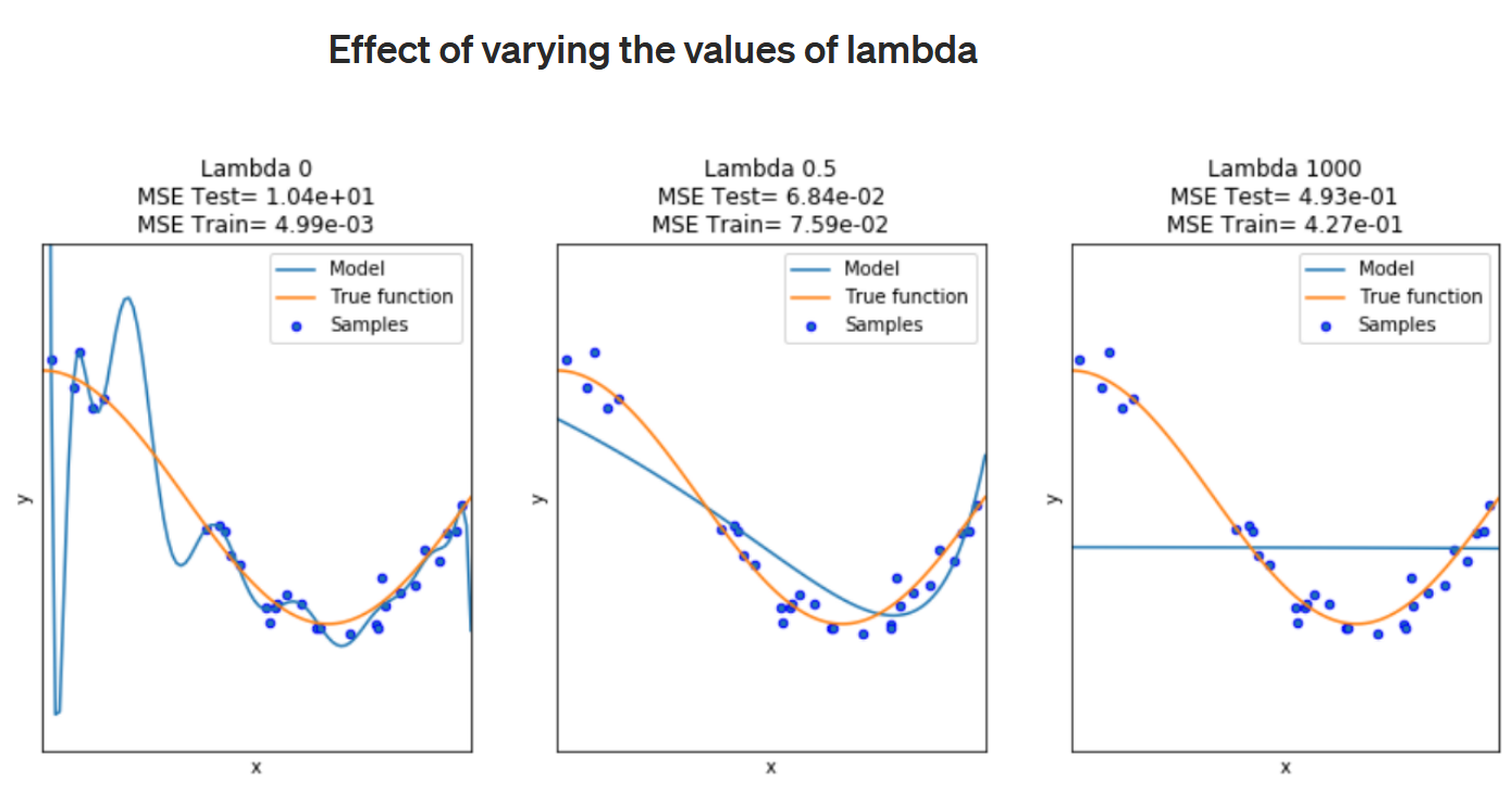
출처: https://towardsdatascience.com/understanding-regularization-in-machine-learning-d7dd0729dde5

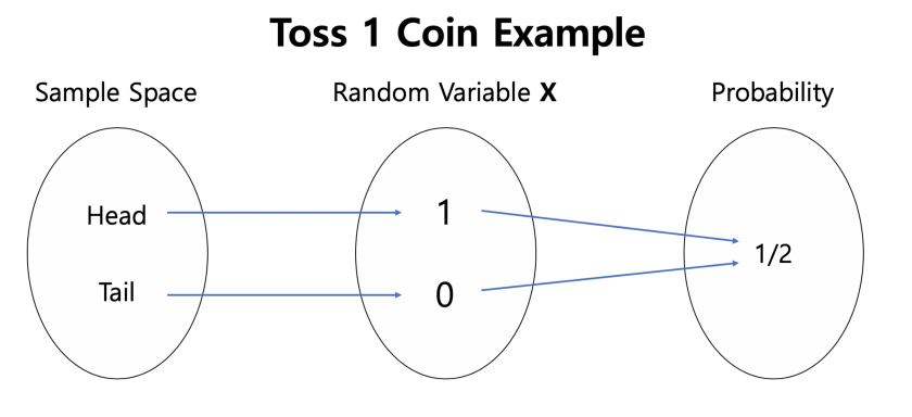
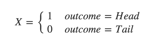
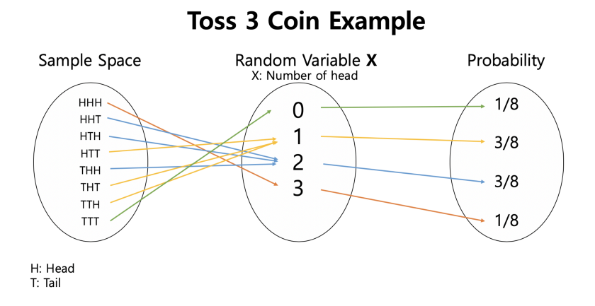
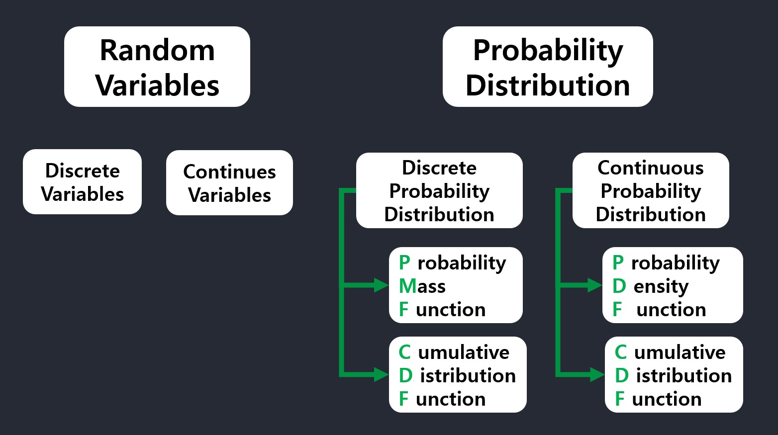
Random Variable

Random Variable: Continuous Random Variable(has PDF, CDF), Discrete Random Variable(has PMF)

Sample space, Random variable X, Probability

Probability Distribution (Discrete Vs. Continuous)

To define probability distributions for the specific case of random variables (so the sample space can be seen as a numeric set), it is common to distinguish between discrete and continuous random variables.

1. Discrete probability distribution

In the discrete case, it is sufficient to specify a probability mass function(PMF) \(p\) assigning a probability to each possible outcome: for example, when throwing a fair die, each of the six values 1 to 6 has the probability 1/6. The probability of an event is then defined to be the sum of the probabilities of the outcomes that satisfy the event; for example, the probability of the event “the dice rolls an even value” is
\[ p(2)+p(4)+p(6) = \frac{1}{6}+\frac{1}{6}+\frac{1}{6} = \frac{1}{2} \]

2. Continuous probability distribution

In contrast, when a random variable takes values from a continuum then typically, any individual outcome has probability zero and only events that include infinitely many outcomes, such as intervals, can have positive probability. For example, consider measuring the weight of a piece of ham in the supermarket, and assume the scale has many digits of precision. The probability that it weighs exactly 500 g is zero, as it will most likely have some non-zero decimal digits. Nevertheless, one might demand, in quality control, that a package of “500 g” of ham must weigh between 490 g and 510 g with at least 98% probability, and this demand is less sensitive to the accuracy of measurement instruments.
Continuous probability distributions can be described in several ways. The probability density function describes the infinitesimal probability of any given value, and the probability that the outcome lies in a given interval can be computed by integrating the probability density function over that interval. An alternative description of the distribution is by means of the cumulative distribution function, which describes the probability that the random variable is no larger than a given value (i.e., \(P(X < x)\) for some x).

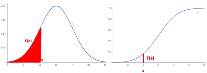
On the left is the probability density function. On the right is the cumulative distribution function, which is the area under the probability density curve. (wikipedia)

Discrete probability distribution

PMF

A probability mass function (PMF) is a function that gives the probability that a discrete random variable is exactly equal to some value.
A probability mass function differs from a probability density function (PDF) in that the latter is associated with continuous rather than discrete random variables. A PDF must be integrated over an interval to yield a probability.
The value of the random variable having the largest probability mass is called the mode.
Well-known discrete probability distributions used in statistical modeling include the Poisson distribution, the Bernoulli distribution, the binomial distribution, the geometric distribution, and the negative binomial distribution. Additionally, the discrete uniform distribution is commonly used in computer programs that make equal-probability random selections between a number of choices.

CDF

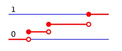
CDF of discrete random variables increases only by jump discontinuities—that is, its cdf increases only where it “jumps” to a higher value, and is constant between those jumps.

Continuous probability distribution

PDF

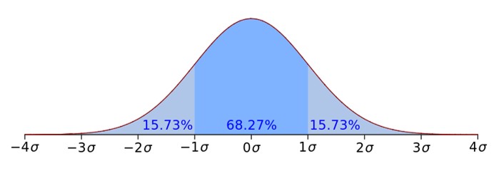
There are many examples of continuous probability distributions: normal, uniform, chi-squared, and others.
if \(I = [a,b]\), then we would have:
\[ P[a \le X \le b] = \int_{a}^{b}f(x)\ dx\]

CDF

\[ F(x) = P[ -\infty< X \le x] = \int_{-\infty}^{x}f(x)\ dx\]

Summary

Appendix

Math Expression(mathjax)

escape

{A}
escape curly brackets using backslash:

\{A\}

tilde

\(\tilde{A}\) :

\tilde{A}

vector norm

\(\lVert \mathbf{p} \rVert\):

$$\lVert \mathbf{p} \rVert$$

white space

a b c:

a\ b\ c\

less than equal to & intergal

\(P[a \le X \le b] = \int_{a}^{b}f(x)\ dx\)

\\[ P[a \le X \le b] = \int_{a}^{b}f(x)\ dx\\]  

Minimal-Mistakes Image center align

default is not allowed for modifying image size sadly. 🤣
using utility class:

![img-alt-title](/assets/images/img.png){: .align-center}

References

regularization: https://daeson.tistory.com/184
lambda: https://towardsdatascience.com/understanding-regularization-in-machine-learning-d7dd0729dde5
random variable: https://medium.com/jun-devpblog/prob-stats-1-random-variable-483c45242b3c https://blog.naver.com/PostView.nhn?blogId=freepsw&logNo=221193004155
https://abaqus-docs.mit.edu/2017/English/SIMACAEMODRefMap/simamod-c-probdensityfunc.htm https://en.wikipedia.org/wiki/Probability_distribution
utility-classes: https://mmistakes.github.io/minimal-mistakes/docs/utility-classes/